
In a previous post I showed How To Turn A Table Into A Column Using Formulas, and in this post we’re going to explore how to do the inverse action and turn a column into a table.

You could do this in a number of different ways but these are the two that make the most sense given a column of data comprised of small blocks of related data like in the example. In this example every three rows of the column relate to one person.
- We could convert this to a table where each column in the table contains the data relating to one person.
- We could convert this to a table where each row in the table contains the data relating to one person.
Option 1
To create a table where each column contains related data we can use this formula.
=INDEX($B$3:$B$14,ROWS($D$3:$G$5)*(COLUMN()-COLUMN($D$3:$G$5))+(ROW()-ROW($D$3:$G$5)+1),1)
$B$3:$B$14 is the original column of data and $D$3:$G$5 is a 4 column and 3 row range because our original data has 4 blocks of related data and 3 items in each block.
Option 2
To create a table where each row contains related data we can use this formula.
=INDEX($B$3:$B$14,COLUMNS($E$11:$G$14)*(ROW()-ROW($E$11:$G$14))+(COLUMN()-COLUMN($E$11:$G$14)+1),1)
$B$3:$B$14 is the original column of data and $E$11:$G$14 is a 3 column 4 row range because our original data has 4 blocks of related data and 3 items in each block.
Formula Breakdown
The INDEX function returns a value from a range based on a row number and column number. So, =INDEX($B$3:$B$14,4,1) refers to row 4 and column 1 of the range $B$3:$B$14, in our example this contains the value Yoda.
Since our range only has one column, the column index in our formula will always be 1 and our formula will look like this =INDEX($B$3:$B$14,number representing the right row,1). We need to be clever about how we get the row number.
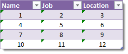
Above are the row index numbers we would like (for option 2) when the formula is copied across the table. Of course, for this formula we will need to know in advance there are 4 blocks of data containing 3 fields each so we can set up the range of our output table as a 4 row and 3 column table. In our option 2 example this table is $E$11:$G$14.
If we want this series of numbers we need a formula like this number of columns in the range * current row of the range + current column of the range + 1. COLUMNS($E$11:$G$14) will give us the number of columns in the range $E$11:$G$14. ROW()-ROW($E$11:$G$14) will give us the current row number (starting at 1) of the range while COLUMN()-COLUMN($E$11:$G$14) gives us the current column number (starting at 1) of the range.
Putting it all together we get our formula for the row index:
COLUMNS($E$11:$G$14)*(ROW()-ROW($E$11:$G$14))+(COLUMN()-COLUMN($E$11:$G$14)+1)


0 Comments