
What It Does
The VLOOKUP function allows you to search a value in the left most column of a range and return the corresponding value in a column to the right. The search is vertical from top to bottom and in fact, the “V” in VLOOKUP stands for vertical.
How It Works

We have a table of data containing a list of student names along with the university they attended, the subject they majored in and their grade average. If I asked you to tell me “what was the major of Reed Gray?” based on the above table of student data, you would likely tell me it was Computer Science. You would be correct, but how did you find this answer?
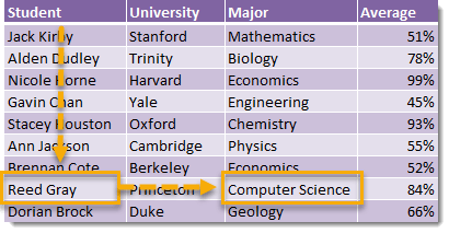
You likely scanned down the first column labeled Student until you found the name Reed Gray, then scanned across the row containing Reed Gray until you came to the Major column and saw that this contained Computer Science. This is exactly how the VLOOKUP function works!
Syntax

- Criteria (required) – This is the item you are looking up in the data.
- Range (required) – This is the range of data which Excel will lookup and return results from.
- Column (required) – This is a positive integer that tells Excel from which column of the Range to return results from.
- Type (optional) – This is a system defined input that tells Excel to return an exact or approximate match. Excel will default to an approximate match if this input is not entered.
- TRUE or 1 – Excel will return an approximate match.
- FALSE or 0 – Excel will return an exact match.
Example
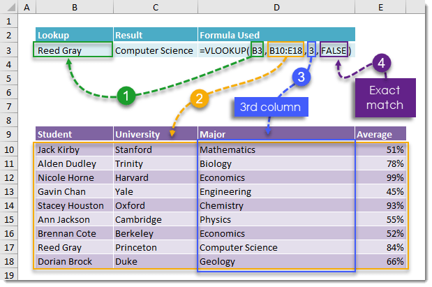
Let’s put VLOOKUP to work and use it to find Reed Gray‘s major!
- B3 – We have entered Reed Gray into cell B3 so this part of our VLOOKUP function will reference this cell.
- B10:E18 – This range contains our table of student data.
- 3 – We want to return data from the Major column and this is the third column to the right of the student column in which we are looking up Reed Gray.
- FALSE – We want to find an exact match so we will use FALSE here.
This will return the result Computer Science.
Duplicate Entries In Our Lookup Column
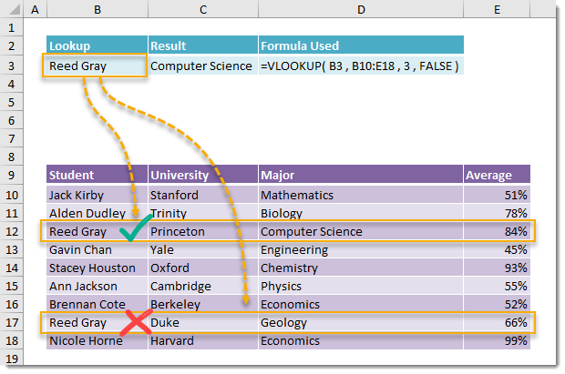
VLOOKUP can only return one value from a set of data and it will return the first match it finds in a list going from top to bottom. If your data contains duplicate items in the column you’re looking up data in, then VLOOKUP will only be able to return the first match.
In the above example, we see Reed Gray is listed twice in the Student column. There is a Reed Gray from Princeton in computer science and a Reed Gray from Duke in Geology. Our VLOOKUP will only return the Reed Gray from Princeton in computer science since this student is listed first in our data.
Lookup From Right To Left
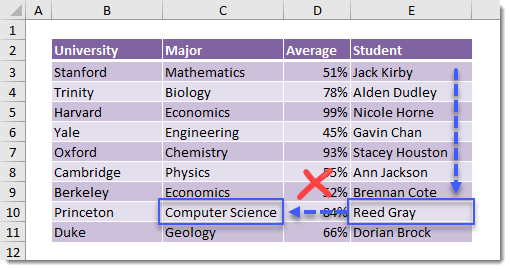
VLOOKUP does not allow you to lookup data from right to left. It will only allow you to lookup data from the left most column of a range and return data in a column to the right.
In the above example our Student column is to the right of our Major column so we will not be able to use VLOOKUP to return a students major.
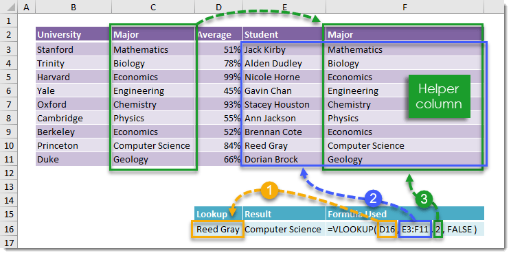
We can overcome this shortfall by using a helper column to the right of our data.
- D16 – This references a cell which contains the item in our data which we want to lookup.
- E3:F11 – This range contains a column from our data plus a helper column to the right which references the Major column.
- 2 – We want to return data from the helper column and this is now the second column from the student column.
- FALSE – We want to find an exact match so we will use FALSE here.
Another option is to combine CHOOSE with VLOOKUP.
Using Approximate Match
Most of the time you are going to want to use an exact match with VLOOKUP, but approximate match can be very useful when dealing with numerical ranges.
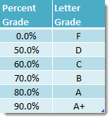
Consider the above table which associates a range of percent grades with a letter grade. We can use this table to get a student’s letter grade based on their percent grade by using a VLOOKUP with an approximate match.
- Under 50% is a F
- 50% up to 60% is a D
- 60% up to 70% is a C
- 70% up to 80% is a B
- 80% up to 90% is an A
- 90% and above is an A+
If we try to use the above table with a VLOOKUP and exact match, any other number between these numbers would result would result in an #N/A error.
With an approximate match, VLOOKUP will find the closest value which is less than the value being looked up. Note that for this to work our table needs to be sorted in ascending order.
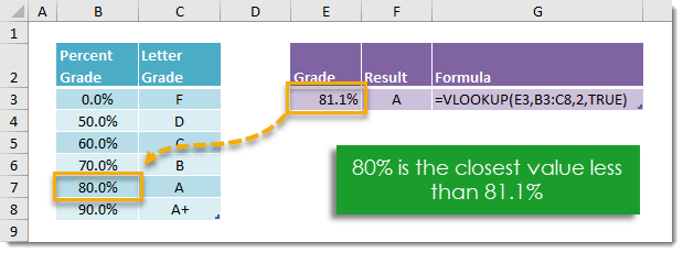
To use an approximate match in VLOOKUP we enter TRUE in the last argument of the function.
Errors From Your VLOOKUP
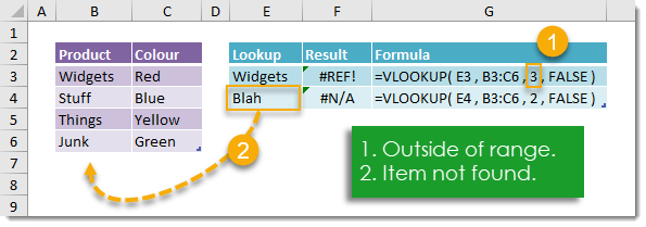
There are two main reason why your VLOOKUP will return an error.
- The column index you’re using is outside of the range selected. This will result in a #REF! error. You can fix this by extending the range to include the column or change the column index to something inside the range.
- The item being looked up is not in your data. This will result in a #N/A error. You can fix this by adding the item to your data or changing what you’re looking up.
If you don’t want to add data to your range but don’t want to see #N/A errors when your VLOOKUP doesn’t find a result then you can wrap your VLOOKUP with an IFERROR. This will return the result “Not Found” instead of #N/A.
VLOOKUP Is Not Case Sensitive
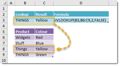
VLOOKUP is not case sensitive. Something like “Things” and “THINGS” are the same to VLOOKUP and the result that is returned will be the top most item in your data.
Use INDEX and MATCH to perform a case sensitive lookup.
Using Wildcards
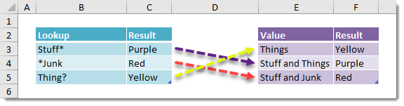
The VLOOKUP function also supports wildcard characters.
- Use * as a wildcard for any number of characters
- Searching for Stuff* will return the corresponding value for Stuff and Things
- Use ? as a wildcard for exactly one character
- Searching for Thing? will return the corresponding value for Things
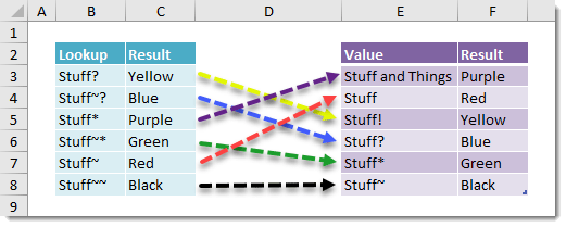
It may be the case sometimes that your data contains the wildcard characters “?” or “*” and we need to look up an item with these characters. In this case we need to use the “~” character in front either “?” or “*” to tell Excel we are not using these as wildcards.
- ~? will search for ?
- Searching for Stuff~? will return the corresponding value for Stuff?
- ~* will search for *
- Searching for Stuff~* will return the corresponding value for Stuff*
- ~~ will search for ~
- Searching for Stuff~~ will return the corresponding value for Stuff~


0 Comments