WARNING!!! Mega POWER Ahead!

Note: When using the completed workbook, you will need to change the folder reference in the query to wherever you save the sample files.

From the Query Editor, go to View > Advanced Editor and change the folder path.

If you’ve ever come across a situation where you’ve had multiple files of data with each file having data spread across multiple sheets then you’ll want to read on.

This post is going to explore how to use the From Folder Power Query to import multiple files with multiple sheets in each file and aggregate the data into one table.

This example has a series of sales files in a folder.

Each file contains the sales for a given country and the files are named according to which country the sales data is from (i.e. Ireland.xlsx, England.xlsx, Luxembourg.xlsx, and Canada.xlsx).

Each file has several sheets with different data in the same format. Each sheet contains the sales for a given salesperson from the country and is named with the sales person’s name.

As you can imagine, aggregating the data manually would be very time-consuming as the number of files and sheets grows. This is where Power Query can shine.

Step 1: Create a From Folder Query

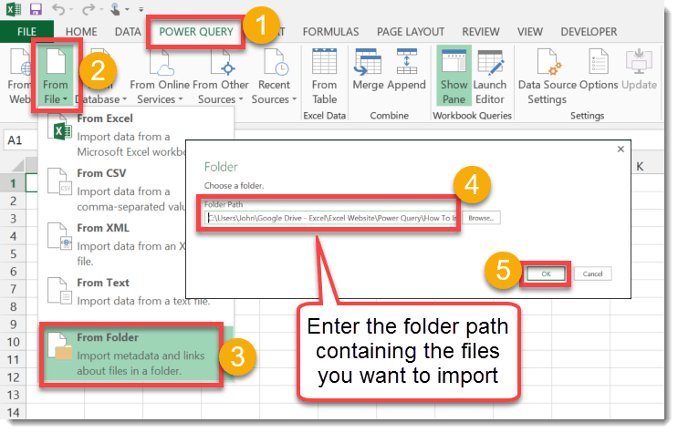
Create a From Folder query.

1. Go to the Power Query tab.
2. Press the From File button.
3. Select From Folder in the drop down menu.
4. Select the folder path of the files you want to import.
5. Press the OK button.

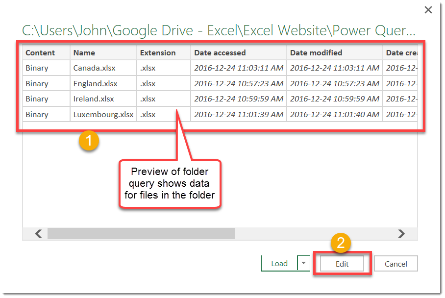
Check the preview data to ensure it is in the correct folder and files.

1. A preview of the import data will appear. Check these are the correct files and folders.
2. Press the Edit button.

Step 2: Remove data columns that aren’t needed

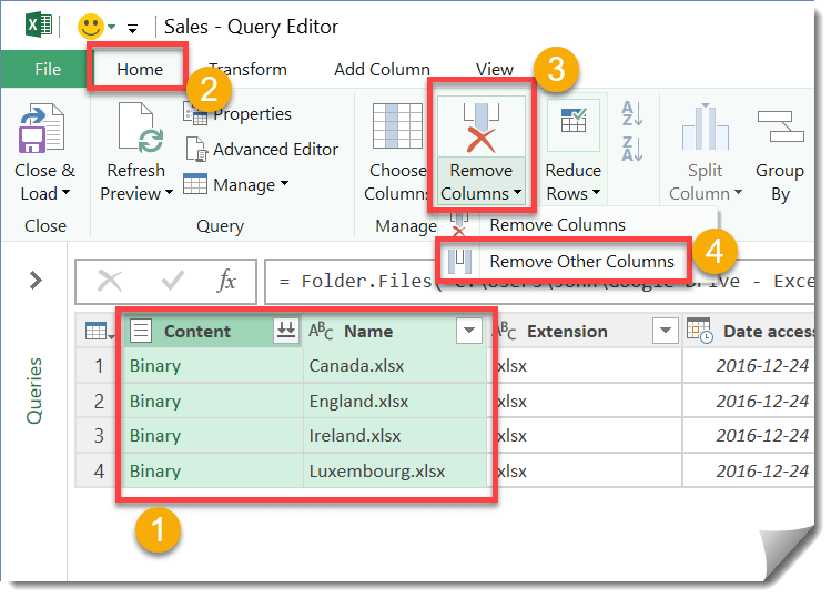
The From Folder query will include a lot of data such as file extension type, date modified, file location, etc.

These are not needed for the purposes of combining data. You can remove these to avoid clutter.

1. Select the two columns you don’t need (Content and Name). Hold the Ctrl key and left click on the column headings to select them.
2. Go to the Home tab.
3. Press the Remove Columns button.
4. Select Remove Other Columns from the drop down menu.

Step 3: Split the file name column

To get the country into the data, you will need to parse the text in the file name.

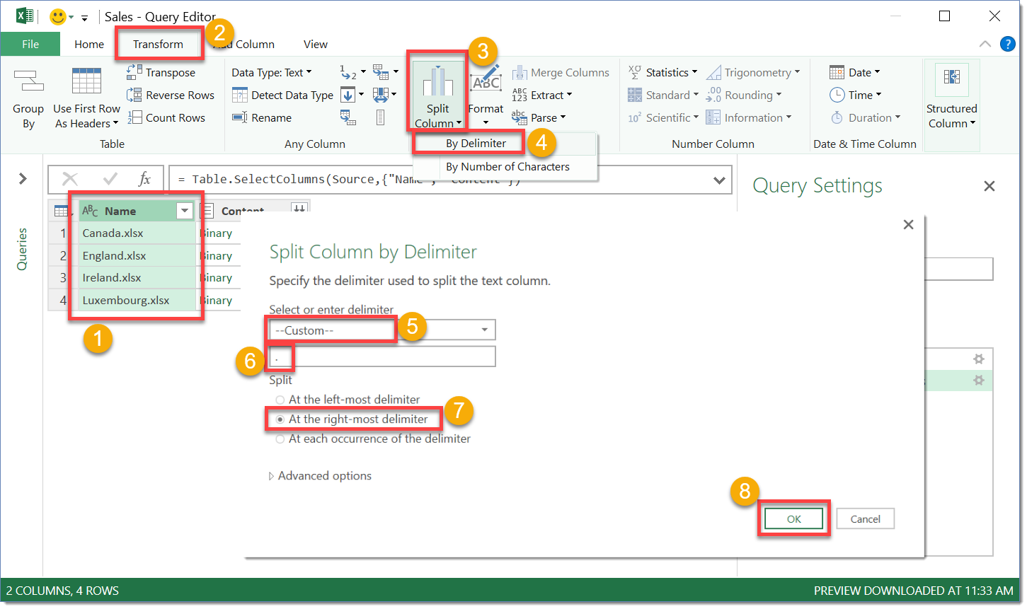
Since the file naming convention is pretty simple (Country Name.xlsx), you can use the split column function using a period as the delimiter.

1. Highlight the file name column.
2. Go to the Transform tab.
3. Press the Split Column button.
4. Choose By Delimiter in the drop down menu.
5. Choose Custom.
6. Enter a period for the delimiter.
7. Choose At the right most delimiter. This will only split the file name text using the right most period found (ie just before the file extention xlsx).
8. Press the OK button.

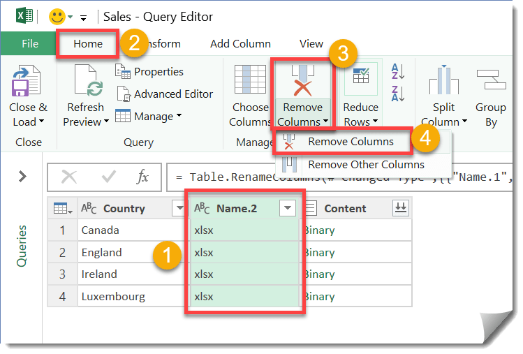
You can remove the resulting column containing the extension part of the split file name.

1. Select the column.
2. Go to the Home tab.
3. Press the Remove Columns button.
4. Select Remove Columns from the drop down menu.

Step 4: Add column for file content

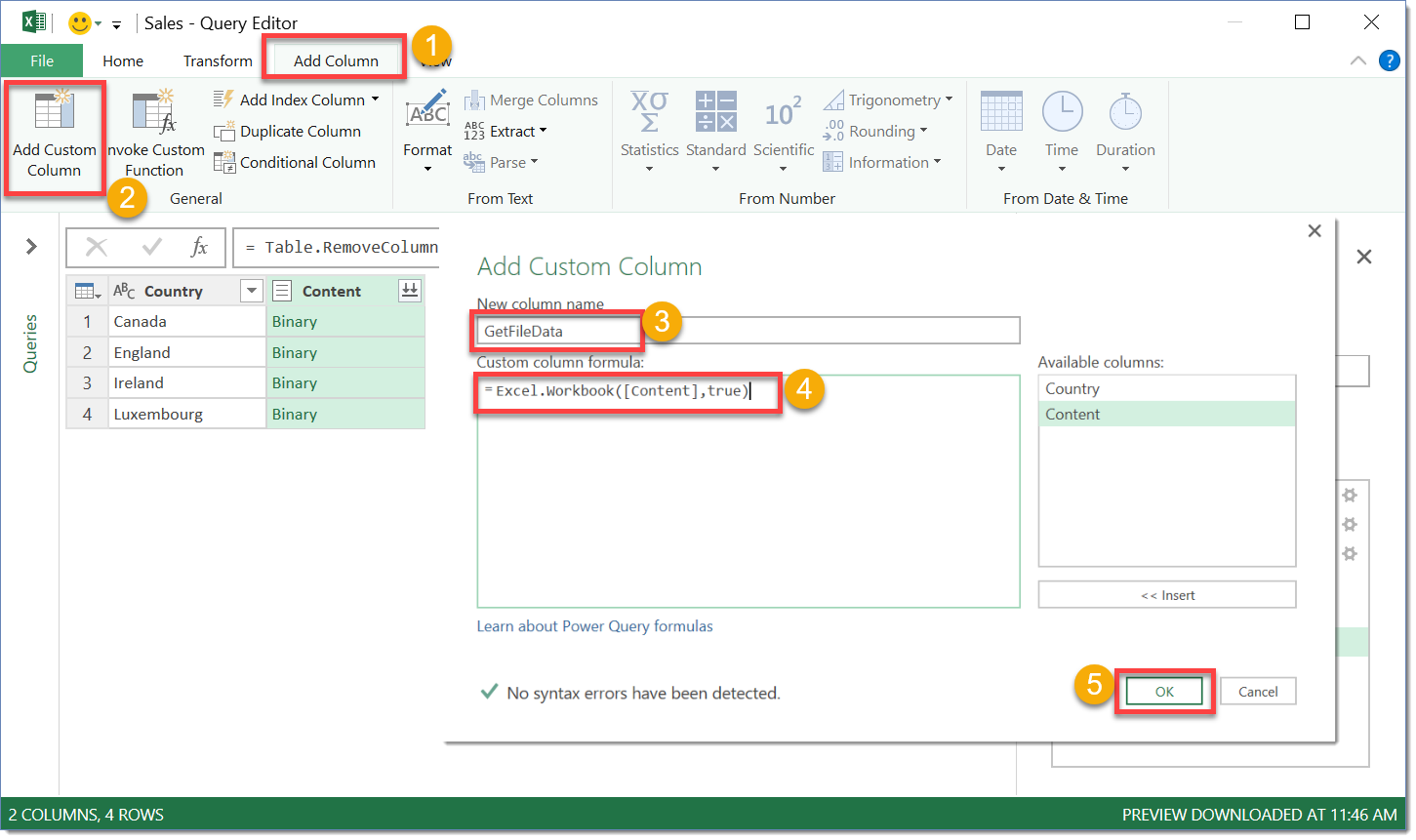
Now you will need to add a column to bring the content into the query.

1. Go to the Add Column tab.
2. Press the Add Custom Column button.
3. Name the new column something like GetFileData.
4. Type this formula Excel.Workbook([Content],true) into the formula area.
5. Press the OK button.

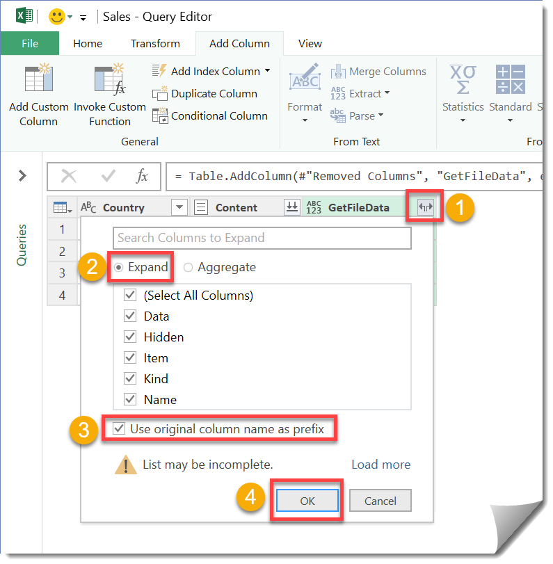
Expand the new column to show all the items in the Content.

1. Press the small double arrow icon in the right hand side of the column heading.
2. Select Expand.
3. Check Use original column name as prefix.
4. Press the OK button.

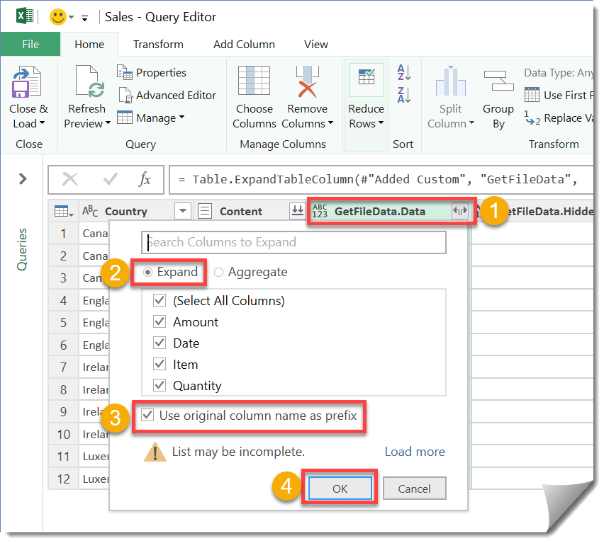
You also need to expand the resulting Data column to show all its elements.

1. Press the small double arrow icon in the right hand side of the column heading.
2. Select Expand.
3. Check Use original column name as prefix.
4. Press the OK button.

Now you have all the columns needed plus a few extra.

Delete any columns you don’t need and rearrange the order of columns if desired by dragging and dropping columns.

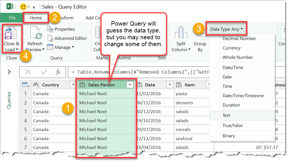
Power Query will guess the data type of each column, but you may need to correct these.

1. Select the column you need to change the data type in.
2. Go to the Home tab.
3. Press Data type and select the data type from the drop down menu.

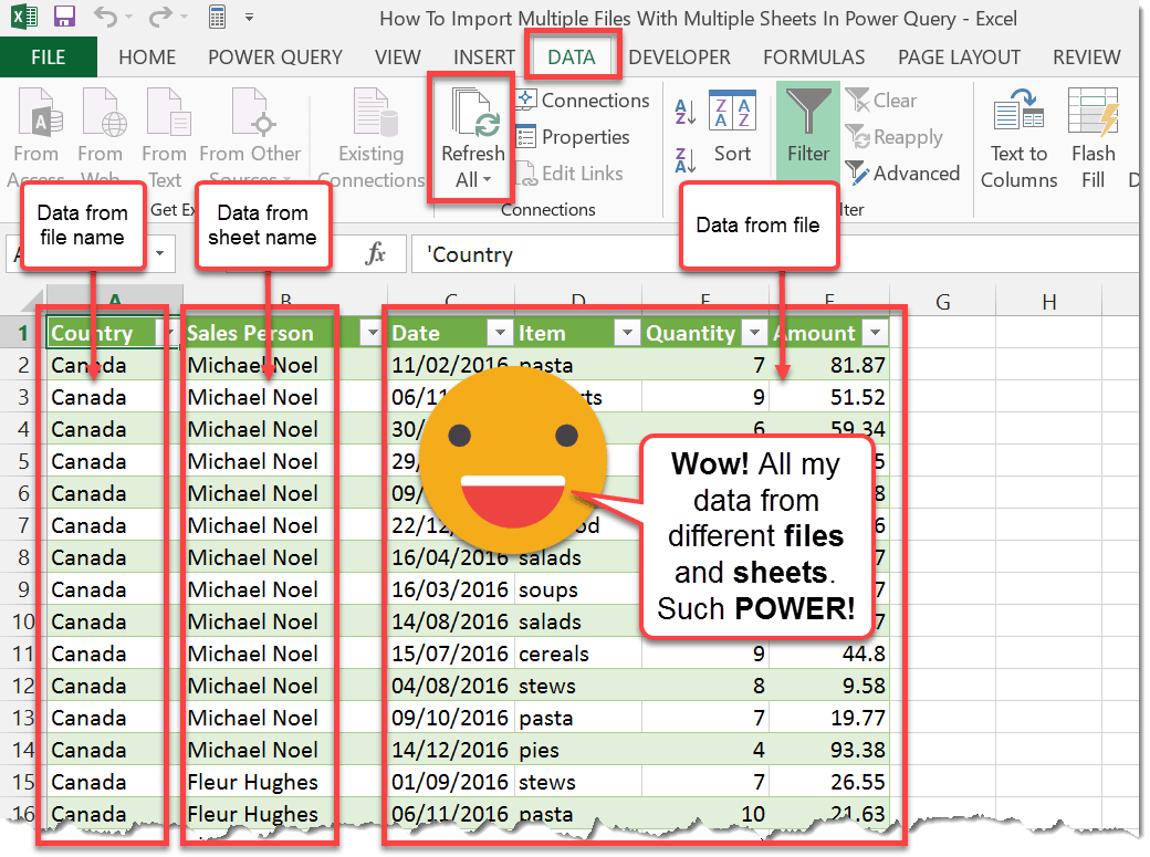
This method allowed you to easily import all the data from multiple files and sheets into one table.

You were also able to add in a country data column based on the file name and a salesperson data column based on the sheet name.

If you add files to the folder or update data in a file, you can easily update the aggregated data by going into the Data tab and pressing the Refresh All button. This will re-run the query to obtain the latest data.

Wow, Power Query can be very powerful!