How To Get A List Of Unique Items From Your Data

I come across this situation a lot, I have a big set of data and I want to quickly see what are the unique values in a certain column. Here are three quick and easy ways to get a list of unique values in your data. Each takes about 30 seconds or less to perform, so you should be well on your way to easy time savings in your work.

Method 1: Advanced Filters

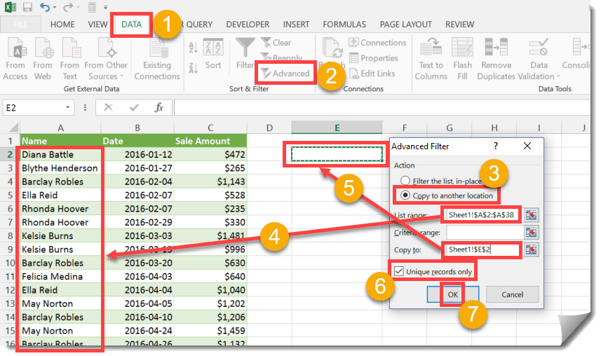
The Advanced Filter has a great feature that allows you to copy a list of unique values from a range you specify to another location.

Go to the Data tab.
Click the Advanced button found under the Sort & Filter section.
Select Copy to another location.
Select the range of values in the List range input which you’d like to see a unique list from.
Select the cell in the Copy to input where you want the values to appear. Make sure there is enough room below this cell as the list start at the this cell and go down.
Make sure the Unique records only box is checked.
Press the OK button.

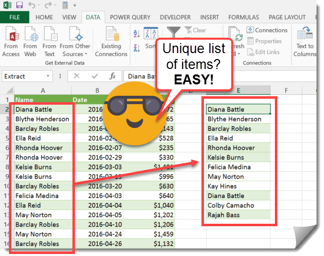
Now your list of unique values will appear starting in the cell you selected. Notice that even format is copied over.

Method 2: Remove Duplicates

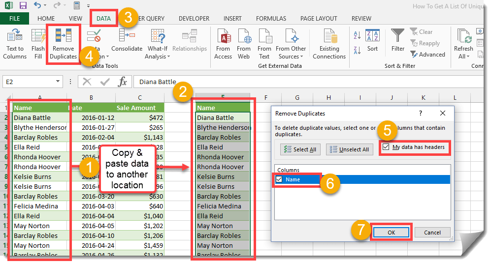
Excel has a very useful feature called remove duplicates which can be used on either the whole data set or a single column of data.

Copy and paste the column of values which you want to see a list of unique values from to another location.
Highlight this list of values.
Go to the Data tab.
From the Data Tools section press the Remove Duplicates button.
If you copied the column heading, then make sure the My data has headers box is checked.
Make sure your column is checked.
Press the OK button.

Method 3: Pivot Table

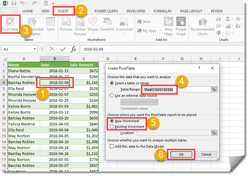
We can also use a pivot table to give a list of unique items.

Highlight any cell in your data.
Go to the Insert tab.
From the Tables section select Pivot Table.
Make sure the selected data range includes all your data.
Select whether you want the pivot table to appear in a New Worksheet, or an existing sheet. If you select existing sheet you will need to select the location.
Press the OK button.

The pivot table method has the advantage that if you add more data the pivot table list of unique items can be refreshed.

About the Author

John MacDougall

John is a Microsoft MVP and qualified actuary with over 15 years of experience. He has worked in a variety of industries, including insurance, ad tech, and most recently Power Platform consulting. He is a keen problem solver and has a passion for using technology to make businesses more efficient.