What questions do we want to answer about our data?

Let’s create pivot tables to answer these questions about our sales data.

• What were the total sales for each sales representative?
• What were the top 3 States for sales?
• What were the total sales for each region by quarter?
• How many of orders were there for each product?

The great thing with pivot tables is it’s easy to answer questions like these about your data with just a few drag and drop actions.

Get The Starting Workbook

Creating a pivot table to answer our questions

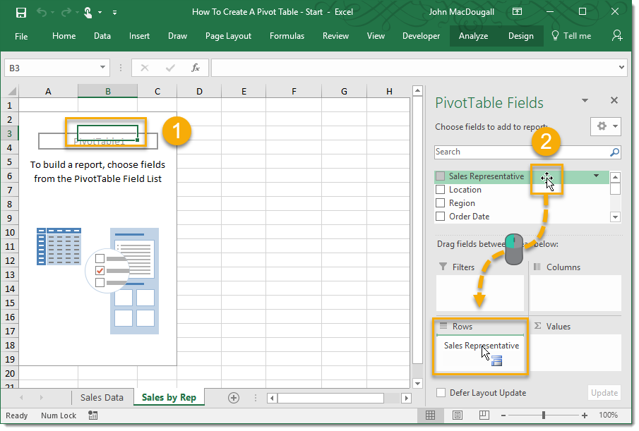
Let’s first make a pivot table to answer what were the total sales for each sales representative? First we will want to add the Sales Representative field to our pivot table.

1. Make sure your active cell cursor is in the blank pivot table previously created here.
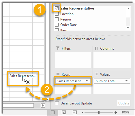
2. Find the Sales Representative field in the PivotTable Fields list and left click to drag and drop it into the Rows area.
   • You can also use the check box to the left of the field name to add or remove a field from the pivot table. By default Excel will add checked fields which contain text values to the Rows area.

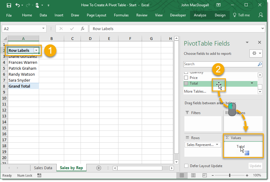
Next let’s add the Total field into our pivot table.

1. Make sure your active cell cursor is still in the pivot table.
2. Find the Total field in the PivotTable Fields list and left click to drag and drop it into the Values area.
   • You can also use the check box to the left of the field name to add or remove a field from the pivot table. By default Excel will add checked fields which contain numerical values to the Values area.

Your pivot table should look something like this and we now have a summary of the Total field for each Sales Representative.

Creating another pivot table

The quickest way to create a new pivot table using the same Sales data is to make a copy of an already existing pivot table. We can do this by either making a copy of the sheet it’s on or by copying and pasting the pivot table to another area in our workbook.

• To quickly copy a sheet
  • Hold Ctrl and then left click and drag the sheet tab over to the right or left and release.
  • You should see a small sheet icon with a plus sign while dragging.
  • Rename the newly copied sheet by double clicking on sheet tab.
• To copy the pivot table
  • Place the active cell cursor inside the pivot table.
  • Go to the Analyze tab.
  • Go to Select then Entire PivotTable from the Actions section.
  • Press Ctrl + C to copy the selected pivot table.
  • Navigate to the area where you want to copy the pivot table to.
  • Press Ctrl + V to paste the pivot table to the new area.

Removing fields from a pivot table

Now we have an exact copy of the pivot table, we can remove any fields we don’t want to use. This can be done in two different ways.

1. Uncheck the box to the left of the field name in the PivotTable Fields list.
2. Drag the item from the Filter, Columns, Rows or Values area to the worksheet area. You will see an X appear with the cursor and you can now release the item to remove it.

Creating a pivot table to show top 3 results

Let’s answer the question what were the top 3 States for sales? Create a pivot table with the Location field in the Rows area and the Total field in the Values area.

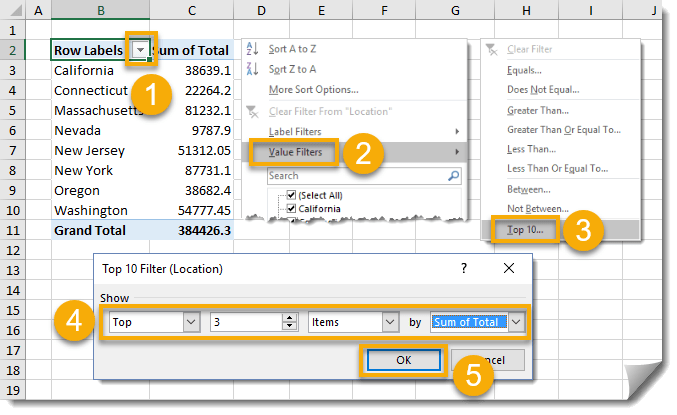
Add a top 3 values filter to your pivot table.

1. Click on the Row Label Filter button in your pivot table.
2. Select Value Filters from the drop down menu.
3. Select Top 10 from the secondary menu.
4. Change the Top 10 Filters window to Top 3 Items by Sum of Total.
5. Press the OK button.

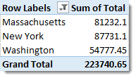
Only the States with the top 3 highest Sum of Total now appear in the pivot table.

Grouping items in a pivot table

Now let’s answer what were the total sales for each region by quarter? Create a pivot table with the Order Date field in the Rows area, the Region field in the Columns area and the Total field in the Values area.

We will need to group our Order Dates into quarters. We could do this in several ways.

1. Add another column to our data and use a formula like this to reference our Order Date and calculate the Quarter it’s in.
2. Use the pivot table Group command.

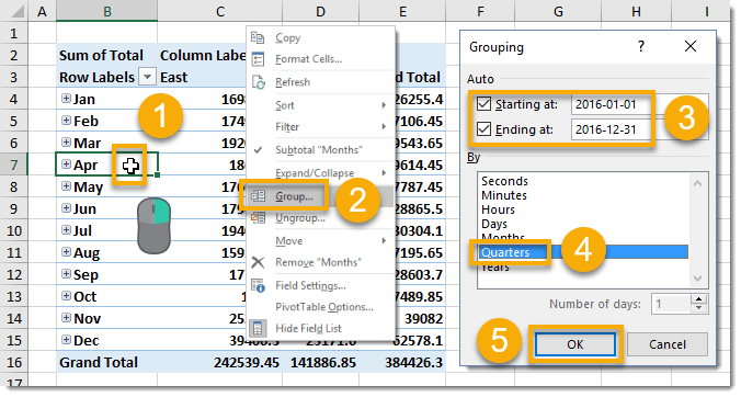
We will use the Group command here. Note that Excel may group these automatically by month as seen above.

1. Right click on any cell in the Order Date column of the pivot table.
2. Select Group from the menu.
3. Make sure the Starting and Ending dates are correct and the range includes all the dates in your data.
4. Select Quarters in the By section of the Grouping window. Remove Months if this was automatically grouped when creating the pivot table.
5. Press the OK button.

Grouping can be used for non-date fields also, but you will need to highlight the items to be grouped together before using the Group command. Hold Ctrl to select non-adjacent cells to be grouped together.

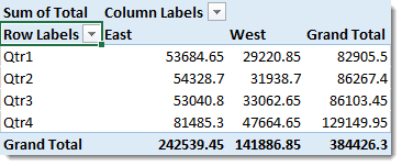
The pivot table will now be grouped by Order Date Quarter in the Rows.

Use a different aggregating method in the values area

So far we have only used the Sum function to summarize our Total field in the Sales data, this is the default when adding a numerical field into the Values area of a pivot table. Pivot table can summarize data in many more ways including Counts, Average, Maximum, Minimum, Standard Deviation, Variance and others. To answer the question how many of orders were there for each product we will need to summarize by Count.

Create a pivot table with the Item field in the Rows area and the Item field in the Values area. Since the Item field is contains text values the aggregation type will default to Count.

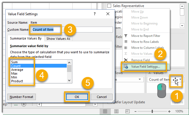
You can easily change the aggregation type for any field in the Values area.

1. Left click on the field in the Values area that you want to change.
2. Select Value Field Settings from the menu.
3. You can also change the Custom Name seen in the pivot table from the Value Field Settings window.
4. Select the aggregation type from the Summarize value field by list.
5. Press the OK button.

Get The Completed Workbook

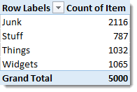
Here we have a Count of orders for each item in our Sales data.