What’s so great about Excel tables? Excel tables are great for organizing and analyzing related data and can make your life a lot easier. They’re definitely a feature you’ll want to start using.

• Formulas that reference a table are easier to read and write when using the table name instead of a generic range address like A2:A10.
• Easily add table styles to your data. These styles (and any formats) are automatically applied to new data (rows or columns) added to the table.
• When you add data to the table formula references automatically update to include this data.
• Each table has it’s own set of filter and sort toggles.
• Column headings and filters automatically stay in view when scrolling down long lists of data.
• Entire columns are easy to select by clicking on the top of the column heading.
• Charts that reference a table will automatically update when you add/change data in your table.
• You can add summary statistics like sums, averages and counts to your table.

Part 1: How to turn your data into a table

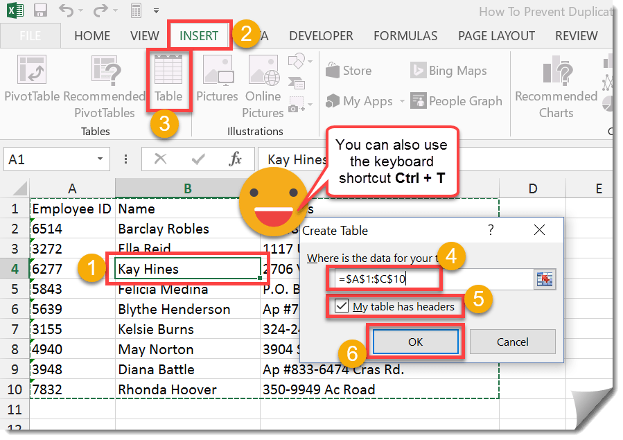
Turn your data into a table.

1. Select a cell in your data range. Any cell will do.
2. Go to the Insert tab.
3. Under the Tables section select Table.
4. Make sure your entire range is selected.
5. Make sure the My table has headers box is checked if the first row of your data has column headings, if not uncheck this.
6. Press the OK button.

You can also insert a table using the Ctrl + T keyboard shortcut.

Part 2: Name and style your table

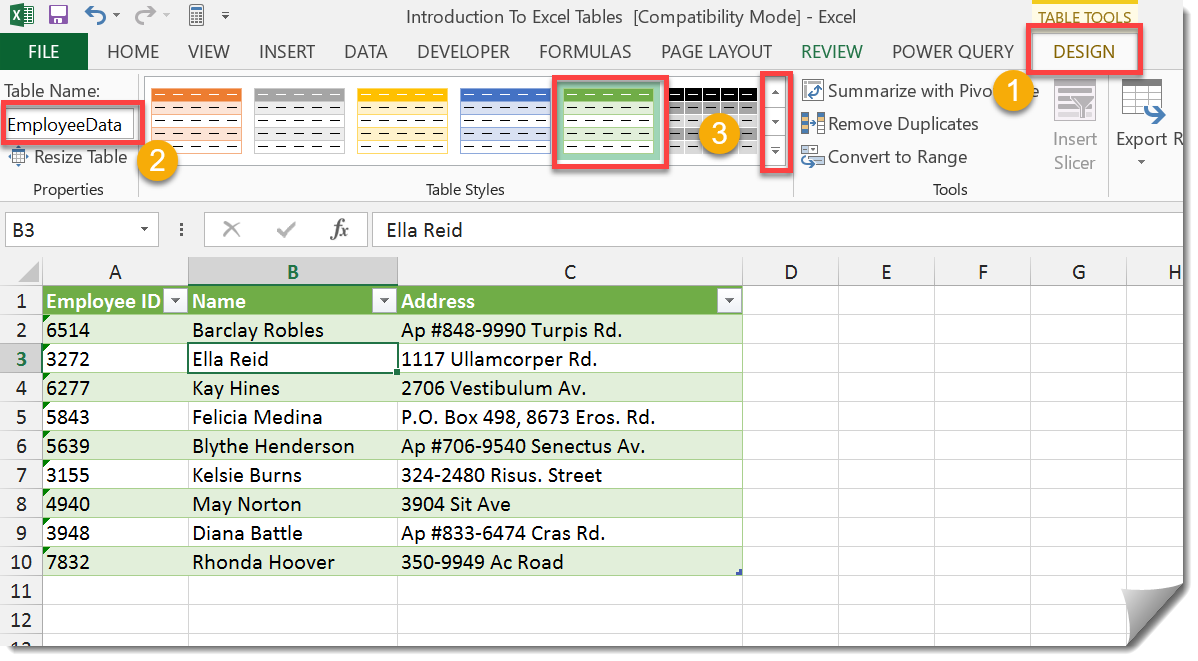
Now that your data has been turned into a table you’ll want to change the default name it’s been given (usually something like Table1) to make it easier to remember when reading and writing formulas that reference the data.

1. Go to the Design tab. This tab is usually only visible when your cursor is on a table.
2. Under the Properties section, type in a new table name that describes what the data is (in this case I’ve named my table EmployeeData) then press enter.
3. Under the Table Styles section, select a table style you like.

Part 3: Adding summary statistics to your table

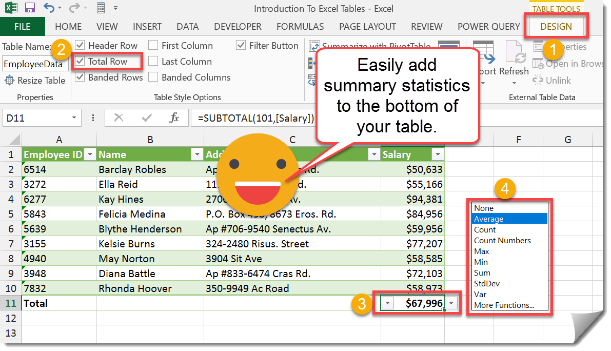
You can easily add summary statistics such as sums, counts and averages to the bottom of your table.

1. Go to the Design tab. This is only visible when your active cell cursor is in a table.
2. Under the Table Style Options check the Total Row option.
3. In the bottom Total row that has been created, select your desired summary formula from the drop down list.

Part 4: Sorting and filtering your table

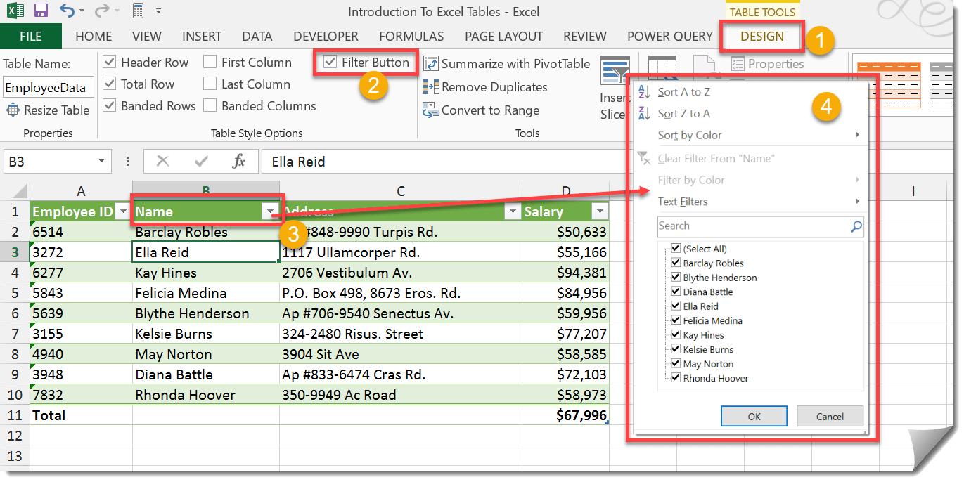
You can also easily sort and filter the data in your table.

1. Go to the Design tab.
2. Make sure the Filter Button is checked.
3. Sort and filter toggles will appear in the column headings of the table.
4. Click the toggle in any column heading to use the sort and filter menu.