There was big news in the Excel world recently. A new replacement for the most famous Excel function was announced.
Move over VLOOKUP, your time in the spotlight is over!
XLOOKUP is here and it can do everything VLOOKUP can do and more!
Let’s take a look at this new function in detail.
Video Tutorial
Problems with VLOOKUP
Why bother introducing a new lookup function? VLOOKUP works just fine, right?
Well, there are a lot of problems with VLOOKUP that a beginner user might not be aware of. When we’re not aware, things can go wrong and we might end up getting incorrect results.
- The VLOOKUP default is not an exact match. The 4th argument in VLOOKUP is optional, but the default is to use an approximate match. This can often lead to incorrect results.
- VLOOKUP can only search from the first to last item and returns the first match.
- VLOOKUP can’t return results from the left, it can only return results to the right of the lookup column. This means we sometimes end up needing to rearrange or add helper columns to our data.
- VLOOKUP needs to reference an entire table. This means we are potentially referencing a lot of cells unnecessarily and this can be very inefficient when recalculating a workbook.
- The lookup column needs to be the first column in our referenced table. Again, this can sometimes mean needing to awkwardly rearrange our data.
- Deleting or inserting columns can break VLOOKUP. The 3rd argument column reference is often entered as a hard coded value. This means if we insert or delete a column the relative position of the return column to the lookup column can change but the hard coded value will not update. This can cause our VLOOKUP’s to return errors or unintended results.
- Approximate match can only return the next smallest item.
- Approximate match needs data sorted in ascending order. Unsorted data in this situation can lead to incorrect results.
XLOOKUP aims to fix these problems.
What Versions of Excel Will Have XLOOKUP?
Only Excel for Office 365 will get the new XLOOKUP function. Excel 2019 and all previous versions won’t ever get this new function.
XLOOKUP is currently only available to those enrolled in the Office Insiders program. But it will eventually become generally available to all Office 365 users.
XLOOKUP Syntax
So what does an XLOOKUP look like? There are 3 required arguments and 2 optional arguments.
= XLOOKUP ( lookup_value, lookup_array, results_array, [match_mode], [search_mode] )- lookup_value (required) – This is the value we want to look up.
- lookup_array (required) – This is the array of values we want to find the lookup_value in.
- results_array (required)- This is the corresponding array of values we want to return results from.
- [match_mode] (optional) – This is the type of match to return. If this argument is not entered, the default will be an exact match.
- 0 = An exact match is returned. If no exact match is found, an #N/A error is returned. This is the default match mode.
- -1 = An exact match is returned. If no exact match is found, the next smallest value is returned.
- 1 = An exact match is returned. If no exact match is found, the next largest value is returned.
- 2 = An exact match is returned, but special characters ?, * and ~ will act as the wildcard characters in a lookup_value allowing us to return partial matches.
- [search_mode] (optional) – This is the type of search to perform. If this argument is not entered, the default will be to search from first to last.
- 1 = Performs the search from the first to last item in the lookup_array and will return the first match from the results_array.
- -1 = Performs the search from the last to first item in the lookup_array and will return the last match from the results_array.
- 2 = Performs a binary search from the first to last item in the lookup_array. Our results_array will need to be sorted in ascending order, or the results may be incorrect.
- -2 = Performs a binary search from the last to first item in the lookup_array. Our results_array will need to be sorted in descending order, or the results may be incorrect.
XLOOKUP Only Requires Three Arguments
XLOOKUP sounds more complicated than VLOOKUP! There are definitely more options available.
99% of the time though, we’ll want to perform a basic exact match lookup. XLOOKUP only needs the first 3 arguments to do this. This makes XLOOKUP more simple than VLOOKUP in this situation.
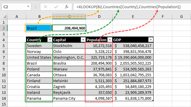
= XLOOKUP ( B2, Countries[Country], Countries[Population] )In this example, we want to return the population for a given country.
We want to find an exact match for the country and return its corresponding population from the table of data.
We only need to use the first three arguments in XLOOKUP to find and return an exact match.
XLOOKUP Can Return Results From The Left
The lookup array and results array are referenced independently. As a consequence, this means XLOOKUP is able to return results to the left of the lookup array.
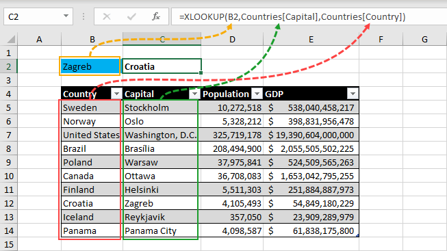
= XLOOKUP ( B2, Countries[Capital], Countries[Country] )In this example, we want to return the country for a given capital city.
This time we place the country column as the results array argument, and we’re able to lookup from right to left with no problems!
XLOOKUP Can Return Horizontal Results
XLOOKUP is also going to replace HLOOKUP, because it can return horizontal results too.
The lookup array and results array don’t need to be vertical. They can be horizontal arrays as well.
In fact, the “X” in XLOOKUP was choosen in part because it works with both vertical and horizontal data.
Bye-bye HLOOKUP!
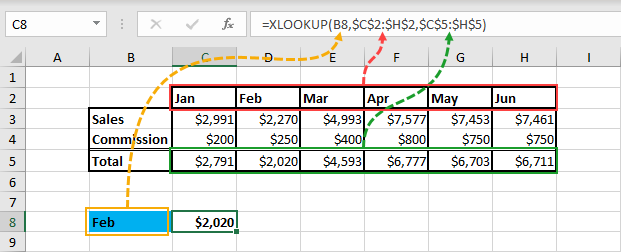
= XLOOKUP ( B8, $C$2:$H$2, $C$5:$H$5 )In this example, we have some month column headings arranged in a horizontal fashion with corresponding values in the rows below.
We can use XLOOKUP to search for a given month and return results from the total row.
XLOOKUP Can’t Do Both Vertical & Horizontal
Since XLOOKUP works with both vertical and horizontal arrays, we might be tempted to try to mix and match them. Unfortunately, this does not work.

= XLOOKUP ( B2, D4:D6, E2:G2 )In this example, we try to perform our lookup in a vertical array and return values from a horizontal array. This results in a #VALUE error.
XLOOKUP Can Return The Next Smallest Or Next Largest Item [Approximate Match]
VLOOKUP’s approximate match could only return the next smallest item in a list. We also needed to have our data sorted in ascending order for this to return correct results.
With XLOOKUP we can choose to either return the next smallest or next largest item. And we don’t need to have our data sorted for this to work.

The 4th argument in XLOOKUP provides us with options to return the next smaller item or the next larger item.
Next Smallest Example
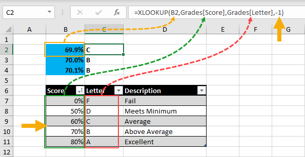
In this example, we are trying to lookup a percentage score and return the corresponding letter grade.
We need to use an approximate match, as the score can be any value from 0% to 100% and we can’t list out all the possibilities.
If we use a -1 in the 4th argument then this will allow us to return the next smallest item.
- Looking up 69.9% will result in a letter grade of C since 60% is the next smallest match.
- Looking up 70% will result in a letter grade of B since 70% is an exact match.
- Looking up 70.1% will result in a letter grade of B since 70% is the next smallest match.
Next Largest Example

Working with the exact same example and switching the 4th argument to 1 will produce the following results.
- Looking up 69.9% will result in a letter grade of B since 70% is the next largest match.
- Looking up 70% will result in a letter grade of B since 70% is an exact match.
- Looking up 70.1% will result in a letter grade of A since 80% is the next largest match.
This isn’t how the grades work, but I didn’t want to come up with a new example 🙂
XLOOKUP Can Search Last To First
It’s pretty well known that VLOOKUP searches first to last and returns the first match. XLOOKUP can do that too.
But XLOOKUP can also search last to first and return the last match.

We don’t need to sort our data in a different order to do this. The 5th argument of XLOOKUP allows us to Search last-to-first.
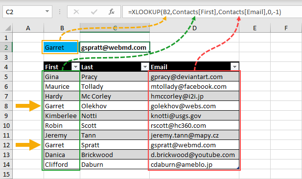
= XLOOKUP ( B2, Contacts[First], Contacts[Email], 0, -1 )In this example, we are looking for a contact’s email based on their first name.
Notice, there are two Garret’s in our list of contacts.
This time, we specify an exact match by using a 0 in the 4th argument. We can then specify to search last to first by using -1 in the 5th argument.
Now XLOOKUP will return the email for the last Garret in our list!
XLOOKUP With Wildcard Characters
VLOOKUP automatically uses Excel’s wildcard characters (*, ?, ~) in its search. This is great if this is your intention, but can be frustrating if you’re trying to search for something that actually contains these characters.
XLOOKUP comes with a wildcard search option in the 4th argument so you can explicitly request a search using wildcard characters.
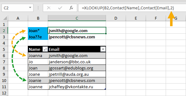
= XLOOKUP ( B2, Contact[Name], Contact[Email], 2 )In this example we use the * and ? character to search for partial matches in a name and then return the corresponding email address.
- Joan* will search for the first match starting with Joan and containing any characters thereafter. This will return jsmith@google.com as the first match.
- Joa??e will search for the first match starting with Joa and followed by any two characters and ending with an e. This will return jpencott@cbsnews.com as the first match.
Search Multiple Criteria With XLOOKUP
We can take advantage of the new calculation engine in Excel along with XLOOKUP to easily lookup based on multiple criteria.
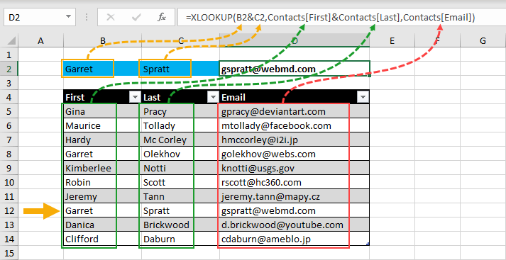
= XLOOKUP ( B2 & C2, Contacts[First] & Contacts[Last], Contacts[Email] )In this example, we want to search for a contact’s email address based on their first and last name. We need to lookup based on two criteria.
We can now use the ampersand character to do this.
We can create a new lookup value based on the first and last name by concatenating them together with an ampersand.
We then need to do the same thing for the lookup array. We create a new lookup array by joining both the first and last name columns with an ampersand.
What Will Happen To VLOOKUP & HLOOKUP?
Now that XLOOKUP has made both these function obsolete, what will happen to VLOOKUP and HLOOKUP?
We will still need to use them if we plan on sharing our workbook with anyone not on Office 365 since XLOOKUP is not available in any other Excel version.
Microsoft won’t be removing them from Excel. They will still be there and available to use. But I could see a time in the distant future when they meet the same fate as the DATEDIF function.


0 Comments