At work this week, I needed to compare two tables to see if the they had similar data. The problem was they were aggregated at different levels with different dimensions and some data in table A was not in table B and some data in table B was not in table A. I needed to find and quantify these differences as well as locate the missing data in each table. I was dealing with ad units, orders, key values, impressions and revenue from the world of online advertising and dealing with 50,000 or so rows of data, but for this post we will look at a more simplified example.

In this example we have table A and table B.

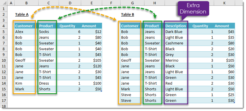
• Table A contains data for clothing purchases by customer and product along with the quantity purchased and the total amount paid. This table has two dimensions of customer and product, and two metrics of quantity purchased and amount paid.
• Table B contains data for the same clothing purchases by customer and product with an extra dimension of description and also includes quantity purchased and the total amount paid. This table has three dimensions of customer and product, and two metrics of quantity purchased and amount paid.

We want to compare these two sets of data and find out where the differences are and quantify these differences. If we take a look at the data we can see some differences.

• Table A contains data for Alex but table B is missing Alex
• Geoff has 2 sweaters in table A but has 3 sweaters in table B

There are several other differences in the tables, but spotting them manually will be hard and won’t scale when your tables have more data. Get & Transform will allow us aggregate these tables to the same level of granularity and join the aggregated data by their common dimensions to easily find the differences.

Get & Transform was previously called Power Query in Excel 2010 and 2013, and you will need to install is as an add-in. Find out how to install Power Query here. If you’re running Excel 2016 then it’s already installed and can be found in the Data tab of the ribbon.

Aggregating The Tables

First we will need to aggregate the data to the customer and product level so that we can compare the two tables.

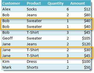
If you look at table A, you will notice that Bob and Jane have rows of data that will need to be aggregated. We ideally want only 1 row of data for Bob and Sweaters and 1 row of data for Jane and T-Shirt.

TIP: I always find it’s a good idea to use Excel Tables with your data. This way, your queries can reference a table name instead of a range. When you add data you won’t need to update the range in your queries as they will reference the name. The data sets in this example have already been turned into tables named Table_A and Table_B, but you can read about how to make a table here.

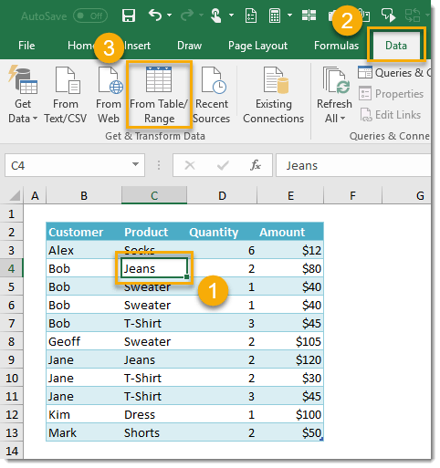
First let’s select our table and make a query.

1. Select a cell in table A or select the whole table.
2. Go to the Data tab in the ribbon.
3. Press the From Table / Range button in the Get & Transform section.

This will open up the Query Editor.

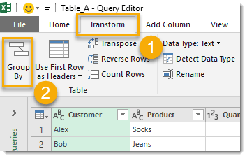
Then select a Group By transformation.

1. Go to the Transform tab.
2. Press the Group By button.

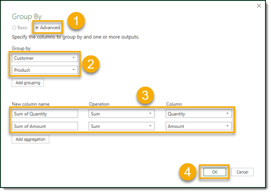
Create your Group By query.

1. Select Advanced to create a Group By query which groups by more than one dimension.
2. Select Customer first and then Product second. You will need to use the Add grouping button to add a second dimension.
3. Add a descriptive column name, select Sum as the Operation for both the Quantity and Amount columns. You will need to use the Add aggregation button to add the second metric.

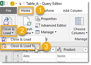
Now save the query.

1. Go to the Home tab in the query editor.
2. Press the Close & Load button.
3. Select Close & Load To.

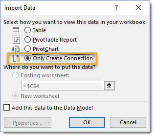
From the Import Data menu select Only Create Connection. We could load this to another table by selecting Table if we want to see this intermediary step in our spreadsheet, but it’s not necessary. We can also select where to load the table to if we do select Table. Press the OK button to finish.

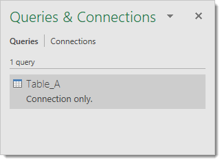
You should now see the Queries & Connections window pane docked to the right of your spreadsheet and it will contain our new Table_A query.

We can repeat the same process to create a Group By query for Table_B with the exact same groupings.

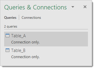
You should now see two Connection only queries in the Queries & Connections window pane for Table_A and Table_B.

Join Queries With Merge

Now we will combine our queries.

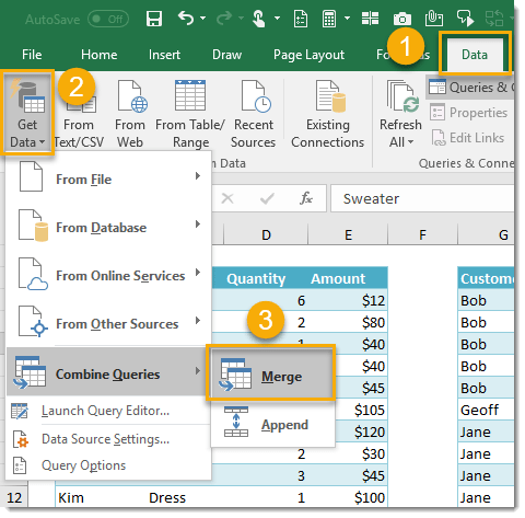
1. Go to the Data tab.
2. Press the Get Data button from the Get & Transform Data section.
3. Choose Combine Queries then Merge from the menu.

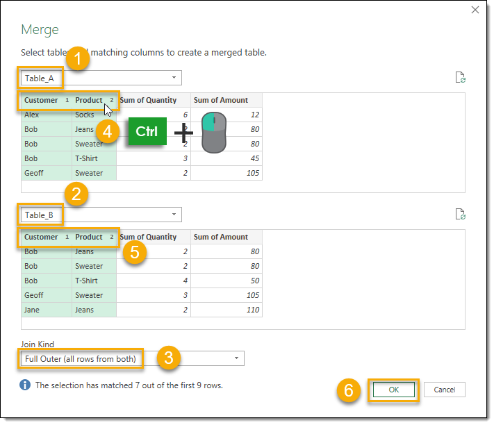
Now we can setup our merge query.

1. Select Table_A for the first query.
2. Select Table_B for the second query.
3. Select Full Outer (all rows from both) for the Join Kind. This will mean all rows in Table_A and all rows in Table_B will be shown in the resulting table.
4. Now we can select which columns our merge query will join on. Hold Ctrl then click on the Customer column and then the Product column. You should see a small 1 next to Customer and a small 2 next to Product.
5. Hold Ctrl then click on the Customer column and then the Product column. We should again see a small 1 next to Customer and a small 2 next to Product.
6. Press the OK button.

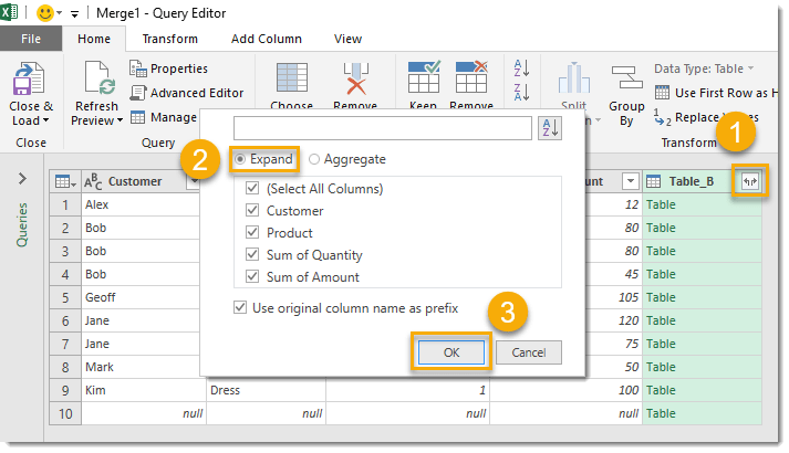
In the editor we will see our Table_A Group By query along with a Table_B column. We will need to expand this column to show the data in our Table_B Group By query.

1. Right click on the expand icon in the right side of the Table_B column.
2. Select Expand.
3. Press the OK button.

Go to the Home tab and press the Close & Load button to create a table of the results in a new sheet.

Compare Data

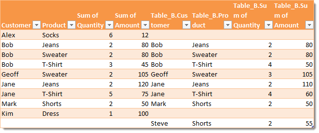
It’s now easy to compare the data in table A and B and see where the differences are.