Pivot tables are awesome! They’re one of Excel’s most powerful features, they allow you to quickly summarize large amounts of data in a matter of seconds. This collection of awesome tips and tricks will help you master pivot tables and become a data ninja!

You’re gonna learn all the tips the pros use, so get ready for a very very long post!

Download the example file with the data used in this post to follow along.

Your Source Data Needs to be in Tabular Format

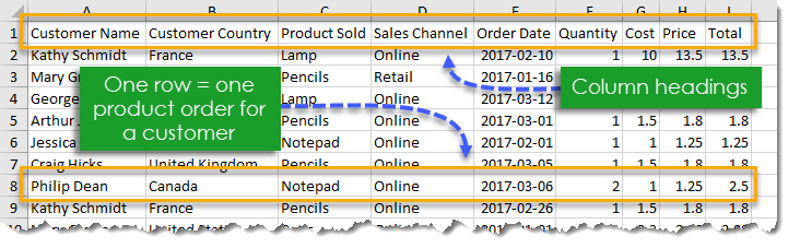
When using a pivot table your source data will need to be in a tabular format. This means your data is in a table with rows and columns.

• The first row should contain your column headings which describes the data directly below in that column. There should be no blank column headings in your data.
• Each row after the column headings should pertain to exactly one record in your data. For example, if your table contains customer data then each row might have the name, street address, postal code and email address for exactly one customer.

Use a Table for Your Source Data

When creating a pivot table it’s usually a good idea to turn your data into an Excel Table. When adding new rows or columns to your source data, you won’t need to update the range reference in your pivot tables if your data is in a Table.

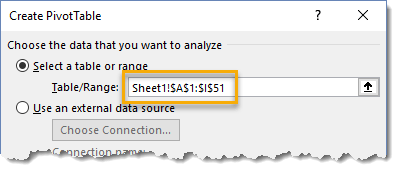
Without a table your range reference will look something like above. In this example, if we were to add data past Row 51 or Column I our pivot table would not include it in the results.

To create and name your table.

1. Select your data.
2. Go to the Insert tab and press the Table button in the Tables section, or use the keyboard shortcut Ctrl + T.
3. Press the OK button.
4. With the active cell inside the table, go to the Table Tools Design tab.
5. Change the Table Name under the Properties section and press Enter.

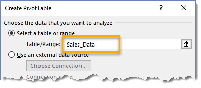
Now when you create a pivot table you can reference it with a name instead of a range. When you add data to the table, you won’t need to update the range in your pivot table. Just refresh it and the new data will appear in your results.

Change Source Data

Ok, if you decide not to use a table for some reason, then you’re going to have to update the range when you add any new rows or columns outside the original range selected.

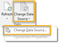
Select your pivot table and go to the Analyze tab and press the Change Data Source button then select Change Data Source from the menu. Update your range accordingly in the following Change PivotTable Data Source pop up dialog box.

Undock the PivotTable Fields Window

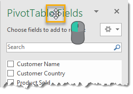
To undock the PivotTable Fields window pane hover your mouse cursor over the title until it turns into a four way arrow, then right click and drag it to your desired location. You can either leave it floating somewhere in the spreadsheet or dock it to the left side by dragging it to the very left edge.

Quickly Dock the PivotTable Fields Window

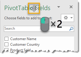
To quickly dock the PivotTable Fields window pane hover your mouse cursor over the title until it turns into a four way arrow, then double right click. It will dock to the last docked location (either to the right or left side).

Hide or Unhide the PivotTable Fields Window

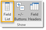
You can get more screen real estate by hiding the PivotTable Fields window. Select a cell in your pivot table and then go to the Analyze tab in the ribbon. Press the Field List button in the Show section to toggle the PivotTable Fields window on or off.

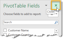
You can also close the window using the X in the upper right corner.

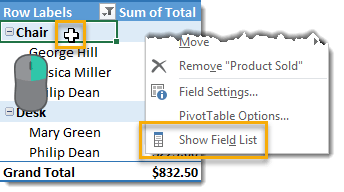
You can also show or hide the PivotTable Fields window with a right click anywhere inside your pivot table then select Show Field List or Hide Field List (depending on the current state of your PivotTable Fields window).

Change the Default Arrangement of the PivotTable Fields Window

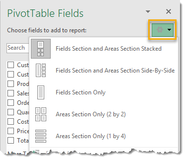
Click on the gear wheel with a downward arrow to change default appearance of the PivotTable Fields window.

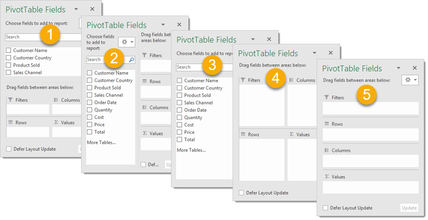
There are five different available options you can select from.

1. Field Section and Areas Section Stacked
2. Field Section and Areas Section Side-By-Side
3. Field Section Only
4. Areas Section Only (2 by 2)
5. Areas Section Only (1 by 4)

Change the Sort Order of Your Field List

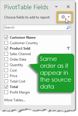
The list of data fields will show in the same order as the source data by default. You can change this to show in alphabetical order (A to Z) if you prefer. Left click on the options menu in the PivotTable Fields window to access the option.

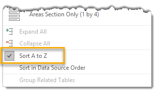
Select the Sort A to Z option in the menu. Your fields will now display in descending order!

Move, Resize and Close the PivotTable Fields Window

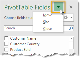
Right click on the small downward arrow to the right of the PivotTable Fields title to move, resize or close the window.

• Move – This will allow you to undock the window and move it around the spreadsheet.
• Size – This allows you to adjust the width and height (when undocked) of the window.
• Close – This allows you to close the window. You can open it again from the Analyze tab > Field List command.

PivotTable and PivotChart Wizard Keyboard Shortcut

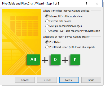
Use the keyboard shortcut Alt + D + P to open the PivotTable and PivotChart Wizard. This will take you through the steps to set up either a pivot table or pivot chart, select your data and the location for your new pivot table or chart.

Create a PivotTable With a Keyboard Shortcut

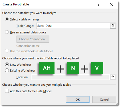
Use the ribbon command keyboard shortcut Alt + N + V to quickly create a pivot table.

Show Details Behind a Value

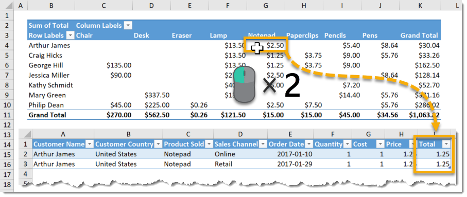
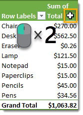
Double right click on a value inside a pivot table to quickly see the data behind that aggregated value. A new sheet will be created with only the data relating to that value.

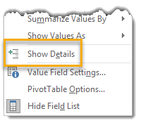
You can also access this feature by right clicking on any value then selecting Show Details.

Turn Off Show Details to Avoid Accidental Double Click

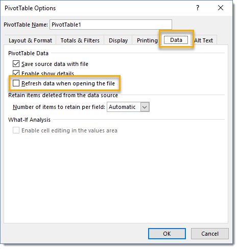
If the ability to show the detailed data behind a pivot table result doesn’t interest you, then you can turn this feature off. This means you and can avoid creating new sheets with bits of data in them because of accidental double clicks.

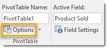
Select your pivot table and go to the Analyze tab in the ribbon. Press the Options button in the PivotTable section to open the options menu.

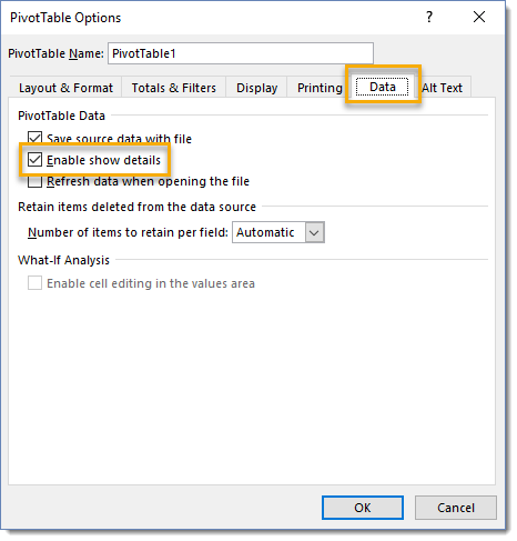
In the PivotTable Options menu go to the Data tab and uncheck the Enable show details box to disable this feature.

Replace Blank Cells

This pivot table contains blank cells because our source data does not contain any records for those combinations of dimensions. For example, there is no data for Arthur James and France so the intersection of the Arthur James row and France column is blank. We can change the settings to display something such as a zero or some text saying “N/A” instead of a blank.

Left click anywhere in the pivot table then select PivotTable Options.

In the PivotTable Options menu

1. Go to the Layout & Format tab.
2. Check the For empty cells show box and enter the value you would like to show for blanks. In our example we will replace blank cells with 0.
3. Press the OK button.

Now the previously blank cells have been replaced by zeros.

Show Items with No Data

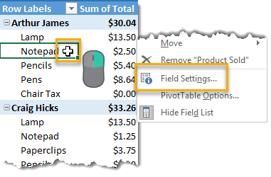
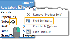
In this example we have create a pivot table with Customer Name and Product Sold in the Rows area. Notice that under each customer, not all the possible products are listed. Only those which we have a transaction in our data are listed. We can change this so that we see all items even when there is no data.

Right click and select Field Settings from the menu.

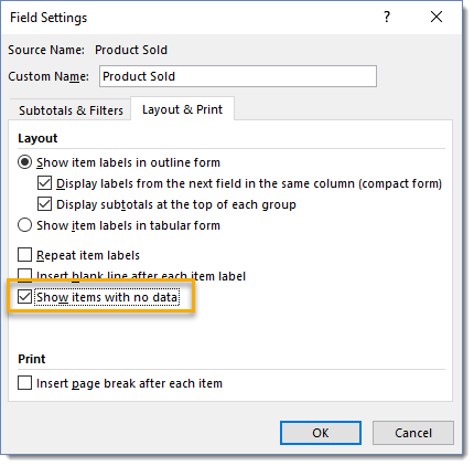
Check the Show items with no data box and press the OK button.

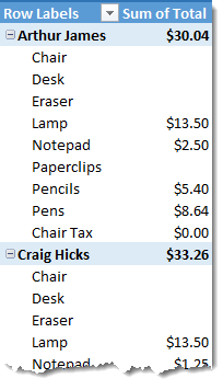
Now we can see all the available items in the Product Sold field even when there is no data.

Remove Items from a Filter Using a Keyboard Shortcut

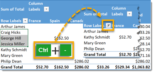
Highlight items in a row or column and press Ctrl + – to remove them from the filter. You can select non-adjacent cells by holding Ctrl and then clicking on the cell.

Add the Current Selection to the Filter

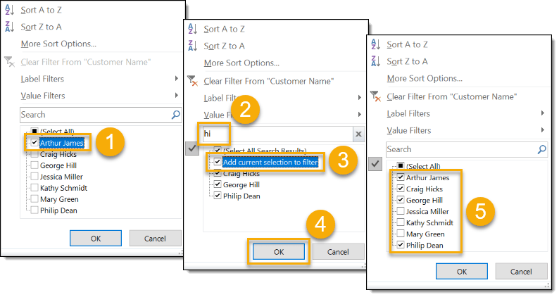
You can use the Search from within a pivot table filter to add items to your previously selected items. This is essentially like using an OR condition in your filtered item searches.

1. Select your first set of items to be filtered on either manually or using the search box (with the same method as step 2 & 3).
2. Use the Search box to search for and then select the second set of items to be filtered on.
3. Check the box marked Add current selection to filter that will appear when using the search box.
4. Press the OK button.
5. Now if you view the filter, you will see both your selections from step 1 and selections from step 2 included in the filter.

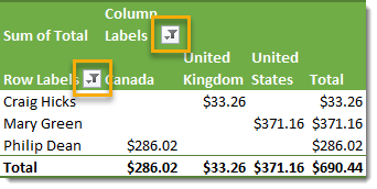
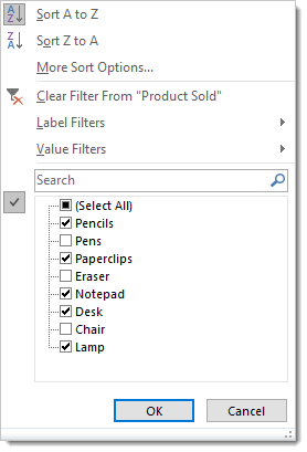
Use the Select All Filter Toggle

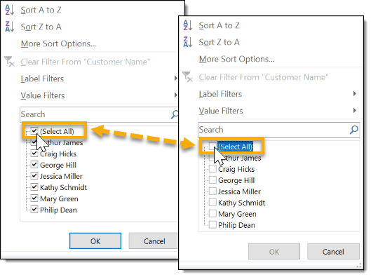
Quickly select or deselect all items in the filter by using the Select All filter toggle. This can be very handy when dealing with a long list of items. You can quickly deselect all and then manually select a small number of items or quickly select all and manually deselect a small number of items.

Defer Layout Update

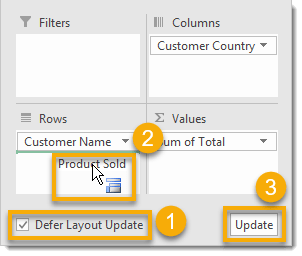
You can defer updating the pivot table while you make changes in the PivotTable Fields window. This is generally only useful if your table is connected to a very large data source and you need to make many changes to the layout. This option is more useful for connections to external data sources as pivot tables with any data you can fit into Excel should be pretty responsive.

1. Check the Defer Layout Update box in the PivotTable Fields window.
2. Make the changes to your layout in the Filters, Columns, Rows or Values section. Your pivot table will remain static.
3. Press the Update button and your table will update to reflect all the changes made.

Add or Remove Fields Using the Check Box

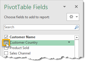
You can quickly add fields to your pivot table by using the check box next to the field name from the field list in the PivotTable Fields window. This can save time if you have a lot of fields to add instead of dragging and dropping each item. Fields containing text data will be added to the Rows section and fields containing numeric data will be added to the Values section when using the check box.

Filter Fields from the PivotTable Fields Window

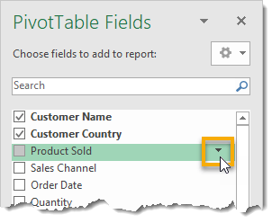
You can filter items in a field from the field list in the PivotTable Fields window. The filter will only apply when the field is added to the filters, columns or rows area. Hover over the desired field and click on the small downward arrow to the right of the field name to open the filter menu.

Rename Any Label

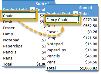
You can rename any label in a pivot table simply by selecting the cell and typing over it. You can change item names in a field, row headings, column headings, filter labels, totals or grand total labels. The only conditions are you can’t rename it to something that already exists in your source data and you can’t type over a value. This doesn’t change the source data, it just changes how the item is labelled.

Rename A Label With A Trailing Space

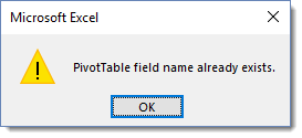
One thing you may want to do is change a column heading like our “Total” column that appears as “Sum of Total” to just show “Total” in the pivot table. Unfortunately, this can’t be done, since “Total” already exists in the source data. If you try to do this you will get a warning pop up saying “PivotTable field name already exists“. We can get around this by adding a space character to the end of the name. This will count as a different name but visually it will look the same as the old field name.

Group Together Items in a Field

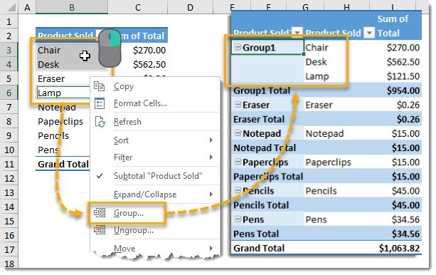
You can group items in a field together to further summarize your data. Highlight the items and then right click and select Group from the menu. You can select multiple non-adjacent field items by holding the Ctrl key while making your selection. By default, the grouped name for a set of items will be Group1, Group2, Group3 etc… But you can change these to something more meaningful.

You can also ungroup a grouped field. Select it and right click then choose Ungroup from the menu.

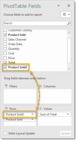
You will notice a new field in appear which has the same name as the grouped field but with a number appended to the end. This is the newly created grouped field and you can use it just like any other field in your data. You can move it to the Filter, Row, Column area or remove it completely from the pivot table. Note that removing it from the pivot table will not ungroup the field.

Group Together Items in a Field Using a Keyboard Shortcut

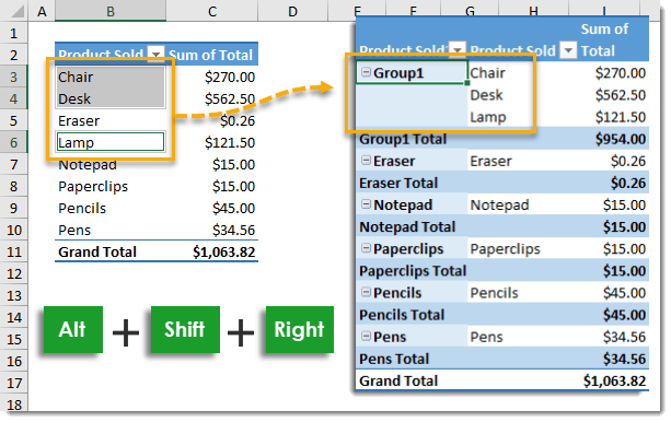
You can quickly group together items in a field by highlighting the items you want to group then pressing Alt + Shift + Right Arrow key.

Ungroup Grouped Items Using a Keyboard Shortcut

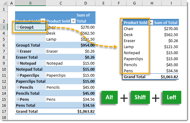
You can quickly ungroup grouped items by highlighting the grouped item and then pressing Alt + Shift + Left Arrow key.

Group Dates

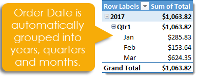
Grouping dates works a little differently than grouping items in a field. When you add a date field into either the rows or columns area, Excel will assume you probably want to view the data by Month, Quarter or Year and will automatically group the dates like this. If you actually wanted the view by date, you will need to right click on it and choose Ungroup from the menu.

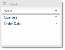
I’ve added the Order Date into the rows area and we can see it’s been grouped by year, quarter and month.

Just like when grouping items in a text field, Excel creates new fields which can be use like any other field. You can remove the original date field without affecting the year or quarter fields.

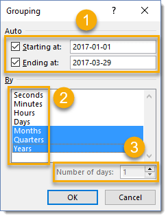
When you right click on the date field and select Group from the menu, you will be presented with a variety of grouping options.

1. You can choose the Starting and Ending dates. All other dates outside the range will be bucketed into a group less than the start date and a group greater than the end date.
2. Choose the levels of granularity for your grouping.
3. If you select only Days as the grouping, you can choose to group based on the Number of days. Choosing 7 would be equivalent to grouping by weeks.

Group Numbers into Ranges

Excel can also group numerical fields. This can be handy if you want to know something like “How much of my sales are from orders less than $50?“.

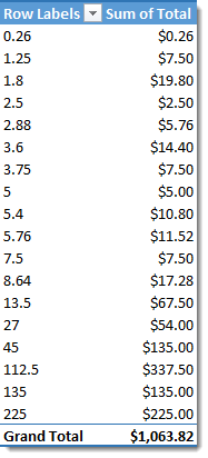
If I place the Total field in both the Rows and Values area, I don’t get anything that useful.

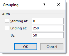
If you right click on the row, this numerical grouping menu will open and you can select a Starting and Ending point along with the interval length.

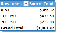
Now it’s easy to see what range most of the sales are in.

Search the PivotTable Fields List

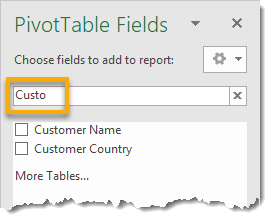
If your source data has a lot of fields then using the search box can help to narrow down the list to find what you’re looking for.

Give Your Pivot Table a Different Style

Quickly change the style of any of your pivot tables using the preset PivotTable Styles.

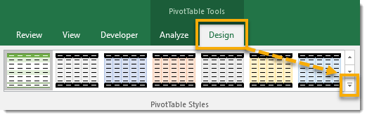
Go to the Design tab in the ribbon and click on the small downward arrow in the PivotTable Styles section to reveal a full selection of pivot table styles available. Note, the Design tab is only visible when the active cell cursor is in a pivot table.

Explore Different Style Options

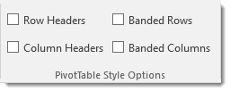
Toggle different PivotTable Style Options on or off. Go to the Design tab in the ribbon and look for the PivotTable Style Options section.

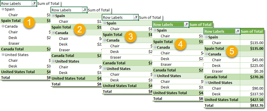
Each option can be independently turned on or off to add a particular style element to your pivot table.

1. With all options unchecked the pivot table is empty of row headers, banded rows, column headers and banded columns.
2. Adding Row Headers.
3. Adding Banded Rows.
4. Adding Column Headers.
5. Adding Banded Columns.

Refresh Your Data

You will need to refresh your pivot table when you add to or change your source data if you want to see these changes reflected in your pivot table results. You can do this from several locations.

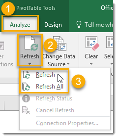
Select a cell in your pivot table to activate the PivotTable Tools tabs.

1. Go to the Analyze tab.
2. Press the Refresh button.
3. Select either Refresh or Refresh All.
   • Refresh will refresh any pivot table connected to the source data of the active pivot table.
   • Refresh All will refresh all data connections for all pivot tables in the workbook.

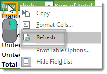
You can also refresh with a Right Click anywhere inside a pivot table and selecting Refresh from the menu.

Refresh with a Keyboard Shortcut

Refresh the connection to the active pivot table’s source data by using the Alt + F5 keyboard shortcut.

Refresh All with a Keyboard Shortcut

Refresh All data connections for all pivot tables in the workbook by using the Ctrl + Alt + F5 keyboard shortcut.

Automatically Refresh Data when Opening Your Workbook

If you want to make sure you’re always looking at the latest data in your pivot tables, you can set the workbook to refresh all pivot tables connected to particular data source. This is especially useful with external data sources.

Select one of the pivot tables connected to your data source then go to the Analyze tab and press the Options button found in the PivotTables section.

From the PivotTable Options menu, go to the Data tab and check the Refresh data when opening the file box. This will refresh all pivot tables in the workbook which are connected to the same data source.

Select the Entire Pivot Table

If you’re like most people, you’ll probably end up making several copies of a pivot table in order to have different views of the data at the same time. If your pivot table is large or has items in the filter area, it can be tricky to select all of it in order to copy and paste. This is when Select Entire PivotTable comes in handy.

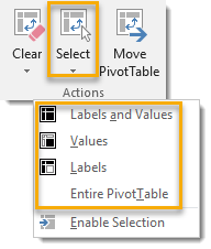
Go to the Analyze tab and press the Select command under the Actions section then choose Entire PivotTable. This will select all of the pivot table including any filter elements above the table.

You can also choose to select only the Labels or the Values area from here.

Clear All Filters

If you have multiple filters engaged on your pivot table you can quickly clear them all without going into each individual filter menu and selecting the Clear Filter From option.

Select a cell in the pivot table which you want to clear filters from to activate the PivotTable Tools tabs in the ribbon.

1. Go to the Analyze tab.
2. Press the Clear button from the Actions section.
3. Select Clear Filters from the menu.

Your pivot table will revert back to a completely unfiltered state showing results based on all source data.

Clear Your Entire Pivot Table

You can clear your pivot tables entirely back to the initial blank state if you want to start over completely with your pivot table analysis.

1. Go to the Analyze tab.
2. Press the Clear button from the Actions section.
3. Select Clear All from the menu.

Your pivot table will now be in its initial blank state with all fields and filters removed.

Clear Old Field Items

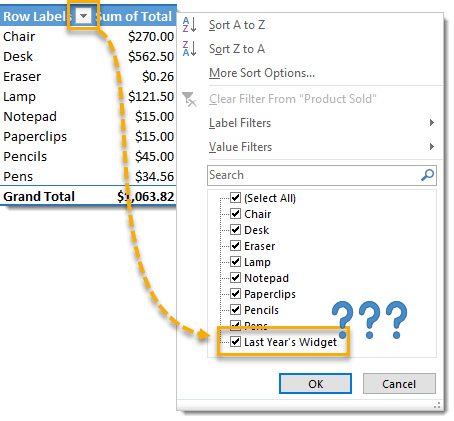
You might have seen this happen before. You delete old data and then add in the new data, but you still see items from the old data after you refresh the pivot table. These items are still stored in the pivot cache and displayed in filter selections even if there is no data for it at all. It can be very confusing when it happens.

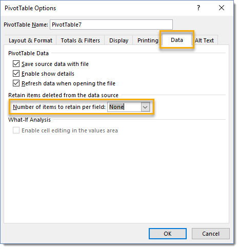
You can change the settings so that your pivot cache doesn’t retain any of the old field items when you refresh your data. Go to the Analyze tab and press the Options button found under the PivotTable section to open the PivotTable Option. Then go to the Data tab and select None under the Number of items to retain per field option.

Now when you refresh, the old phantom items will no longer appear.

Format Numbers

Unfortunately, number formatting from source data does not transfer into your pivot tables. You may want to format your numbers to make them more readable.

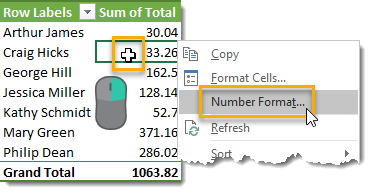
To format a given field, Right Click on any number in that field and select Number Format from the menu. The familiar Format Cell dialog box will open with only the Numbers tab available and you will be able to format the numbers in your field the same as any other cell in your workbook.

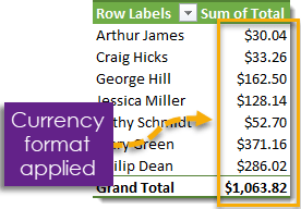
The cool thing is that applying your number formats this way will be dynamic. Even when you move the field around in the pivot table, add other fields or filter on items the formatting will remain applied to the entire field in the pivot table.

Expand or Collapse Field Headings

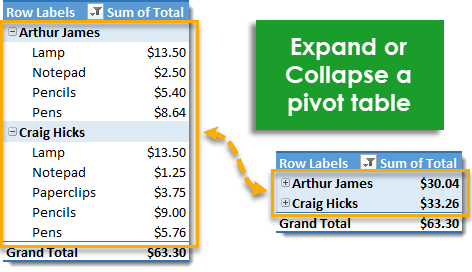
If your pivot table has multiple dimension fields in a row or column you can expand or collapse the outer fields to show more or less detail.

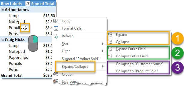
Right click on the field you want to expand or collapse and select Expand/Collapse from the menu.

1. You can expand or collapse only the selected item and leave the remaining alone.
2. You can expand or collapse every item in the field selected.
3. You can expand or collapse only the selected item to a given level.

Double Click to Expand or Collapse Field Headings

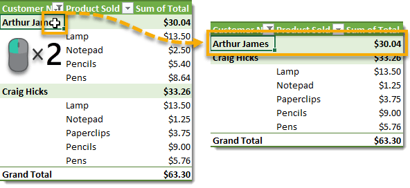
You can expand or collapse fields with a double right click on the field item. This is great to de-clutter a pivot table when you only need to show the full detail for one item.

Add or Remove Expand or Collapse buttons

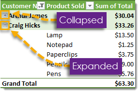
You can add expand or collapse buttons to your pivot tables to make it more obvious to another user that they can expand or collapse the pivot table view as well as which items are already expanded or collapsed.

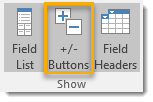
To add these buttons, select your pivot table and go to the Analyze tab and press the +/- Buttons button in the Show section.

Automatically Create a Pivot Table for each Item in a Filter

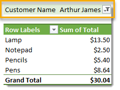
Let’s say you have a pivot table with a field in the Filter area and you would like a pivot table for each item in the field. You might think this has to be done manually by copying the pivot table and then filtering on a new item in the field, but this can actually be done automatically using Show Report Filter Pages. In our example we have the Customer Name field in the filter area and pivot table is currently filtered on Arthur James, and we want a pivot table like this for each customer.

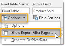
Select you pivot table, it will need to have a field in the filter area. Go to the Analyze tab in the ribbon and press the Options button found in the PivotTable section then select Show Report Filter Pages from the menu.

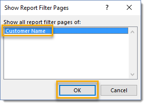
Select the desired field from the Show Report Filter Pages dialog box if you have multiple fields in the filter area of your pivot table then press the OK button.

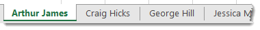
Excel will now create a new sheet for each item in the field you selected. Each sheet will be named after the item in your field and will contain a copy of your pivot table filtered on that item. It’s a big time saver when you have a lot of items in your field.

Allow Multiple Filters Per Field

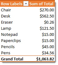
Excel has two types of filters available for a pivot table field, Label Filter and Value Filter. Let’s say you wanted to filter this pivot table on all Product Sold that start with “P” (using a Label Filter) and having a Total value larger than $20 (using a Value Filter), with the default settings this is not possible to have both filters at the same time. We can update the settings to allow this.

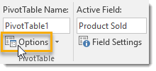
Select your pivot table and go to the Analyze tab in the ribbon and press the Options button in the PivotTable section.

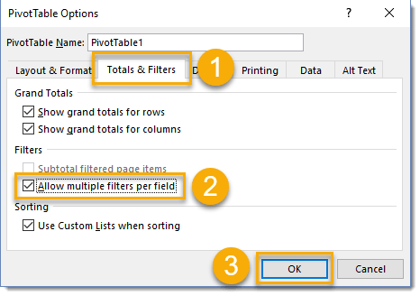
Enable multiple filters in the PivotTable Options dialog box.

1. Go to the Totals & Filters tab.
2. Check the Allow multiple filters per field box.
3. Press the OK button.

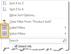
Now you will be able to use both Label Filter and Value Filter at the same time on one field.

Get a List of Unique Values from a Field

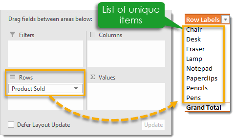
You can use pivot tables to get a list of the unique values in any field of your data. Simply drag the field which you want unique values from into the Rows area of a blank pivot table and the resulting pivot table will contain a list of unique values from your data for that field.

Count the Occurrence of an Item in a Field

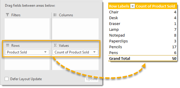
Placing any field with text data into the Values area of the pivot table will cause the calculation to default to Count instead of Sum. This means we will get the count of the number of occurrences of each item. In this example, we have placed Product Sold field which contains text data, into both the Rows and Values area of the pivot table, and we see Count of Product Sold in the Values area.

Delete Your Source Data

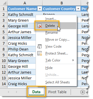
After creating your pivot table you can delete the source data if you want to reduce the workbook file size. You can delete your source data by deleting the sheet it’s contained on. Right click on the sheet tab and select Delete from the menu. Your pivot table contains a cache of the data so it will continue to work as normal. If you want to see your data again you can double left click on the grand total of your pivot table and the data will appear in a new sheet.

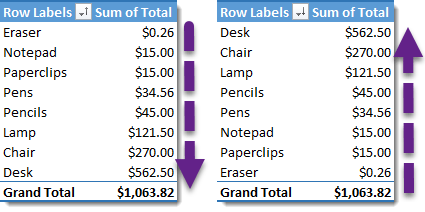
Sort Items Alphabetically in Ascending or Descending Order

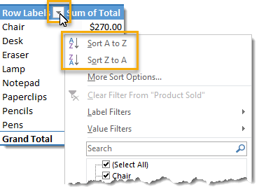
Sort items alphabetically in either ascending or descending order. Left click on the filter icon and select Sort A to Z for ascending or Sort Z to A for descending order.

Manually Sort Items

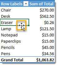
Select the item you want to move and hover your mouse cursor over the active cell border until it turns to a four-way arrow cross.

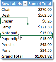
Left click and drag the item to its new position. You will see a large green bar that indicates where the item will be placed.

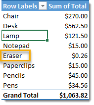
Release the item into its new position.

Sort Items According to a Corresponding Value

You can sort your pivot table by ascending or descending values.

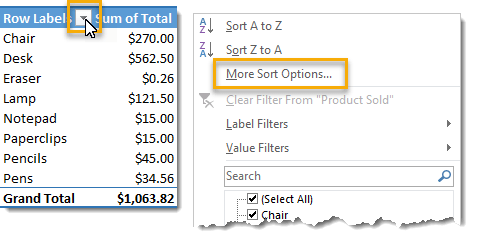
From the filter menu select the More Sort Options.

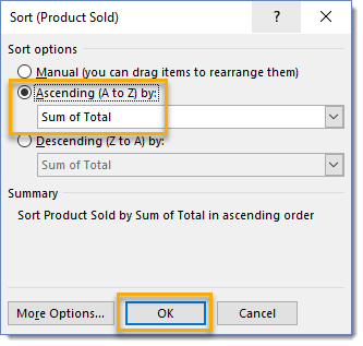
Select either Ascending (A to Z) or Descending (Z to A) then choose one of the value fields in your pivot table and then press the OK button.

Create a Custom Sort Order

If sorting a field alphabetically in ascending or descending order doesn’t suit your needs, you can create a custom sort order by creating a custom list!

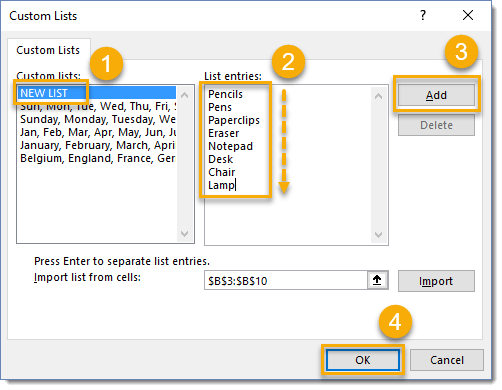
To add a custom list, go to the File tab in the ribbon and select Options. From the Excel Options menu choose Advanced then scroll down to the General section and press the Edit Custom List button.

1. Select NEW LIST from the Custom lists box.
2. Enter your list of field items appearing in the order you want them to sort in your pivot table.
3. Press the Add button to add your list.
4. Press the Ok button.

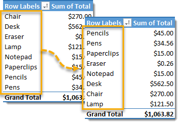
Refresh your pivot table and the order will change to that of the list you entered. This will also be the default sort order now for that field any time you create a pivot table with that field in it.

Insert Blank Line After Each Item

For a less cluttered look and feel you can insert a blank line after each item in your pivot table. Select your pivot table and go to the Design tab of the ribbon and click on the Blank Rows button in the Layout section then select Insert Blank Line after Each Item.

Items in your pivot table will be visually separated with white space so the viewer knows that the data pertains to something different. You can get rid of these blank rows from the Design tab of the ribbon and clicking on the Blank Rows button in the Layout section then selecting Remove Blank Line after Each Item.

Double Click to Open Value Field Settings

You can double right click on any column heading to open the Value Field Settings for that field.

Count Distinct Items

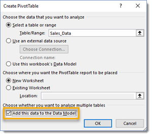
To count distinct items you will need to create your pivot table with data added to the Data Model. Check the Add this data to the Data Model box when creating your pivot table.

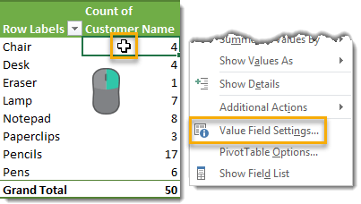
In this example, we have our Product Sold field in the Rows area and Customer Name in the Values area which gives us a count of the orders by product. If we want a unique count of the customers who ordered each of the products then we need to change the default Count to Distinct Count for our values settings. Right click anywhere on the field which you want to obtain a distinct count for and then select Value Field Settings from the menu.

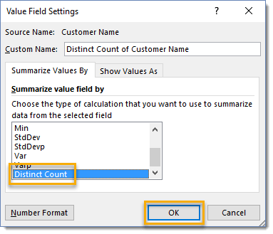
From the Value Field Settings select Distinct Count to summarize value field by and press the OK button.

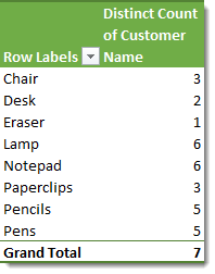
Now the values will display the distinct count. Note the Grand Total now reflects that we have 7 distinct customer names in our data of 50 orders.

Hide Selected Items

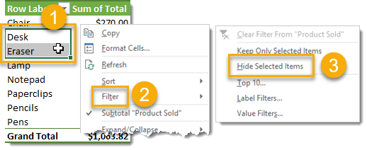
You can hide selected items quickly without going into the filter menu (small down arrow next to the column heading).

1. Select the items you want to hide with your filter. You can use Ctrl to select non-adjacent items. Then right click on the selected items.
2. Select Filter from the menu.
3. Select Hide Selected Items from the sub menu.

This allows you to quickly filter out items without going into the filter menu and checking or unchecking boxes in a long list of items.

Keep Selected Items

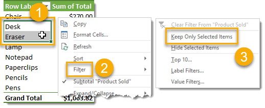
Similarly to hiding selected items, you can choose to keep only the selected items with a filter.

1. Select the items you want to keep with your filter. You can use Ctrl to select non-adjacent items. Then right click on the selected items.
2. Select Filter from the menu.
3. Select Keep Only Selected Items from the menu.

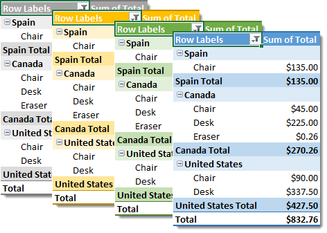
Change the Layout

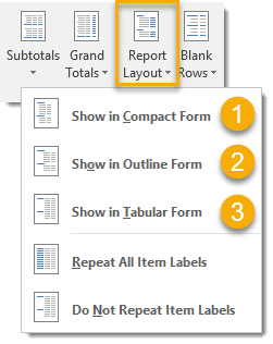
To change the layout of your pivot table go to the Design tab and select Report Layout button under the Layout section. You can select from three different layout options.

1. Show in Compact Form
2. Show in Outline Form
3. Show in Tabular Form

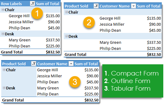
To demonstrate the different layout options, we have created a pivot table with two fields (Product Sold and Customer Name) in the Rows section and a field (Total) in the Values section.

1. Compact form will contain all the Row fields in one column in a hierarchical structure.
2. Outline form will still have a hierarchical structure but each Row field will be in a separate column in the pivot table.
3. Tabular form will not be in a hierarchical structure and each Row field will be in a separate column in the pivot table.

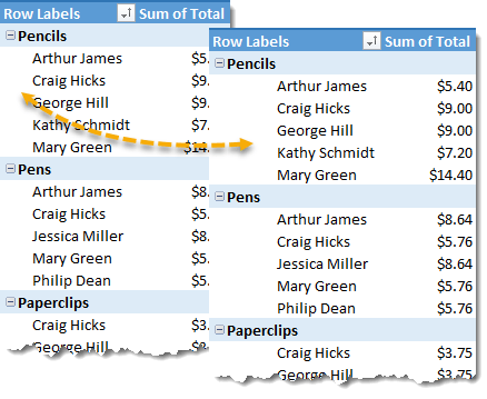
Repeat All Item Labels

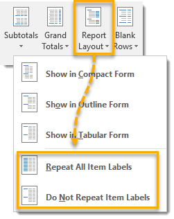
You can repeat all your pivot tables item labels by going to the Design tab and selecting the Report Layout button under the Layout section. Select Repeat All Item Labels to turn on repeated labels and select Do Not Repeat Item Labels to turn off repeated labels.

By default, a pivot table will show the field label and then blank cells underneath for all other sub-fields included in the field heading. Creating a Tabular Form layout with Repeat All Item Labels is a great way to create another set of more aggregated “Source Data” that you can copy and paste as values and use elsewhere.

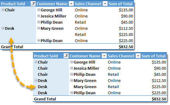
Turn Grand Totals On or Off

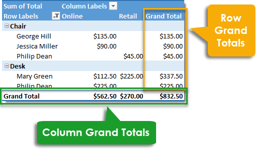
You can add grand totals to your pivot table to help you see at a glance the total for any values field across any row or column.

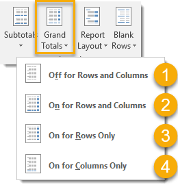
Go to the Design tab and select the Grand Totals command from the Layout section. Select from the four option for displaying grand totals.

1. Off for Rows and Columns (no grand totals will display)
2. On for Rows and Columns
3. On for Row Only
4. On for Columns Only

Turn Subtotals On or Off

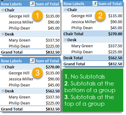
When your pivot table has more that one dimension, you can add or remove subtotals to make results easier to understand.

1. No subtotals results in a cleaner looking pivot table, but you lose vital information about totals across parent level field grouping.
2. Adding subtotals below the group results in extra rows in your pivot table.
3. Adding subtotals above the group results in the extra information but without the extra rows (with a compact layout).

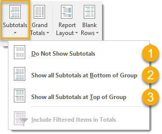
Go to the Design tab and select the Subtotals command from the Layout section. Select from three option for displaying subtotals in your pivot table.

1. Do Not Show Subtotals
2. Show all Subtotals at Bottom of Group
3. Show all Subtotals at Top of Group

Turn Off GETPIVOTDATA

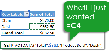
By default when you try to reference a cell within a pivot table in a formula, Excel will create a GETPIVOTDATA formula for the reference. These can be annoying when you want a simple relative A1 style reference since the GETPIVOTDATA acts similarly to an absolute reference.

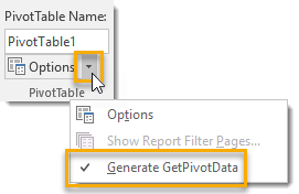
You can turn this default option off by selecting your pivot table then going to the Analyze tab in the ribbon and clicking on the small down arrow next to the Options button under the PivotTable section. Uncheck the Generate GetPivotData option to turn this feature off. You can also turn it back on from there too!

Add a Second Field to the Values Area

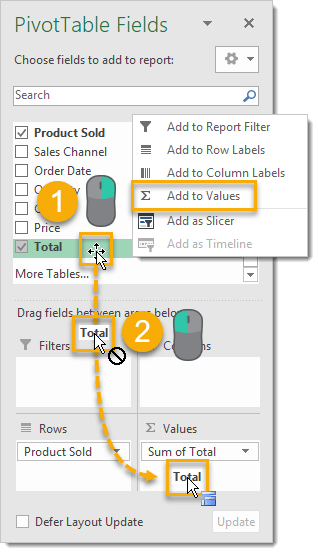
You can add the same field to the Values area of your pivot table two or more times.

1. Right click on the field you want to add to the Values area again and select Add to Values.
2. You can also left click and drag the field into the Values area again.

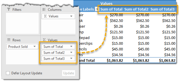
Each time you add the field to the Values area it will get a sequential number added to the end, but remember you can change these titles. You can then change the summarize type to show a Count, Average, Max, Min, Variance or Standard Deviation instead of the Sum. This will allow you to summarize the field in a variety of different ways at the same time.

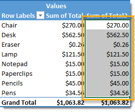
Add Data Bars

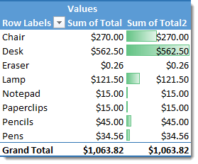
Adding data bars can be a great way visually show the relative value of each item in your pivot table. In the above table we’ve added the Total field to the pivot table twice and used one instance to add data bars to the pivot table.

Select the range in your pivot table where you’d like to add the data bars.

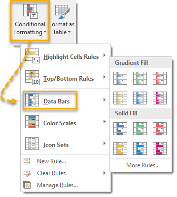
Go to the Home tab in the ribbon and under the Styles section press the Conditional Formatting button then select the Data Bars option from the menu. You can choose either a Gradient Fill or Solid Fill and there are several different color options available. You can also create your own style data bars using the More Rules options in the menu. The cool thing is these data bars will be dynamic and applied to the entire field even if the range changes when you add dimensions or update data.

Add Color Scales

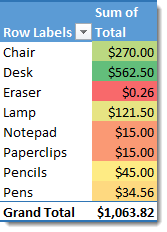
You can add color scales to your pivot table to create a heat map to easily identify high, medium and low values in your data.

Select the range in your pivot table where you would like to add the color scales.

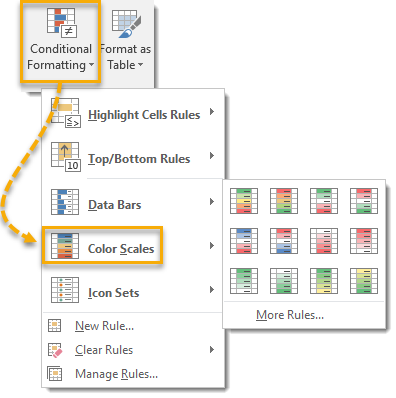
Go to the Home tab and under the Styles section press the Conditional Formatting button then select the Color Scales option from the menu. There are several different color options to choose from or you can create your own rules and color options by selecting More Rules.

Add Icon Sets

You can add various icon sets to your pivot tables to visually indicate items that increased, decreased or stayed the same.

Select the range in your pivot table where you’re wanting to add the icons.

From the Home tab and in the Styles section press the Conditional Formatting button and then select the Icon Sets option. You’ll find a large variety of icon options to choose from including arrows, shapes, flags, checks and X’s, stars and many others. You can adjust the rules for when each symbol appears by using the More Rules option.

Add Highlighted Cells Rules

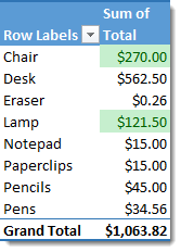
You can add conditional formatting to highlight cell values that fit certain rules to make them stand out. In this example I have created a rule to highlight cells between $100 and $300. You can create many different types of rules.

• Numbers greater than a given value.
• Numbers less than a given value.
• Numbers between two given values.
• Numbers equal to a given value.
• Text that contains a specific string.
• Dates that meet a given criteria.
• Duplicate values.

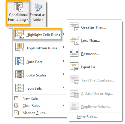
Go to the Home tab and in the Styles section select Conditional Formatting then select the Highlight Cells Rule option. You can then select from the options mentioned above and set the criteria values required.

Add Highlighted Top or Bottom N Formatting

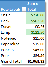
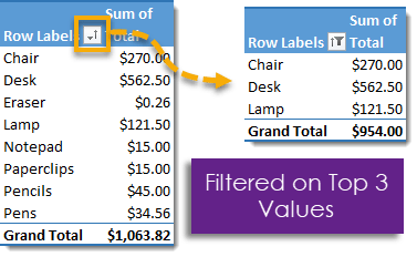
You can add conditional formatting to highlight cells that are in the top N or bottom N values of the pivot table. In this example I have added the formatting to show the top 3 values. Choose from several different options.

• Top 10 items.
• Top 10 percent.
• Bottom 10 items.
• Bottom 10 percent.
• Above average.
• Below average.

Although these options mention top and bottom 10, the number can be selected as desired.

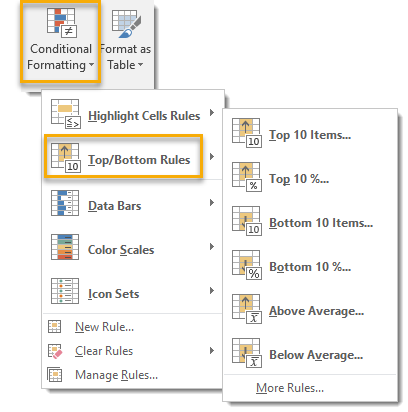
In the Home tab and under the Styles section select Conditional Formatting then select the Top/Bottom Rules option. You can then select from the options mentioned above.

Format Numbers as Invisible Text

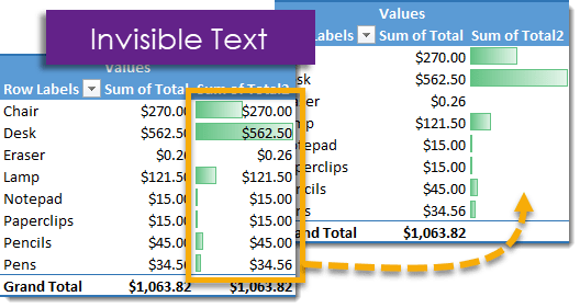
If you’ve added some sort of conditional formatting like data bars to your pivot table and want to get rid of the numbers to clean up the look of the table, then you can format the numbers as invisible text.

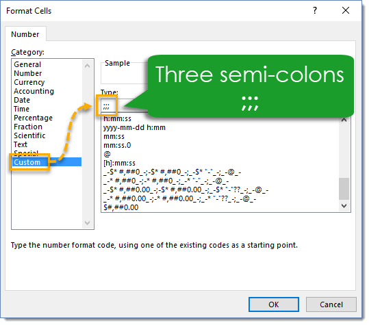
Right click anywhere in the field which you want to format and select Number Format from the menu. In the Format Cells dialog box choose Custom from the Category and then type three semi-colons ;;; into the Type area and press OK. The data will still exist in your pivot table, but it just won’t be visible!

Use Conditional Format Settings to Remove Text

When you add data bars or icon sets with conditional formatting, there is actually a setting to show only the data bars or icons. This can be found in the More Rules menu when setting up your conditional formatting.

This is a more simple option than messing around with custom formats, but is limited to data bars and icons.

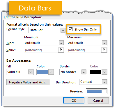
For the data bars check the Show Bar Only box.

For the icon sets check the Show Icon Only box.

Prevent Column Width Changing on Update

By default Excel will automatically adjust columns of a pivot table so that everything fits. This means those really long headings like Count of Customer Country will take up a lot of column space. If you adjust these wide columns to a smaller size, the next time you update the pivot table they will auto adjust back to fit the long heading title. You can change the settings so this doesn’t happen.

Open the pivot table option. Select your pivot table and go to the Analyze tab in the ribbon then press the Options button in the PivotTable section.

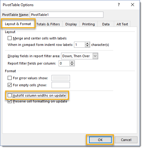
In the PivotTable Options window under the Layout & Format tab uncheck the Autofit column widths on update box. This will allow you to make changes to your pivot table without the column width automatically adjusting.

Add A Calculated Field

Adding a calculated field to your pivot table is equivalent to adding a new column to your source data to perform a calculation based on the other data. For example, our data contains a Total Cost and Total amount for each order. If we want to calculate the Profit Margin on each order we could add another column with the calculation Profit Margin = 1 – (Total Cost / Total) or we can add calculated field.

For a rate type calculations like a profit margin, it’s better to add the calculations as a Calculated Field rather than add an extra column with the calculation to the source data. Adding a rate calculation to the source data may result in incorrect calculations in your pivot table when viewing a pivot table at a more aggregated view than the data. Always add a calculated field instead!

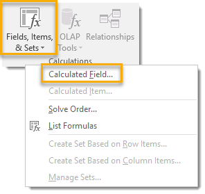
Select your pivot table and go to the Analyze tab in the ribbon and press the Fields, Items & Sets button found in the Calculations section. Then select Calculated Field from the menu.

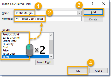
Add your calculation in the Insert Calculated Field dialog box.

1. Give your new calculation a Name. This is the field name that will appear in the pivot table.
2. Create your Formula. You can double right click any field in the field list to use it in your calculation.
3. Press the Add button.
4. Press the OK button.

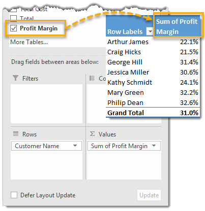
Your calculated field will appear in the PivotTable Field list and can be used to create your pivot table just like any other field.

Removing A Calculated Field

You can delete a calculated field by selecting your pivot table by going to the Analyze tab in the ribbon and pressing the Fields, Items & Sets button then selecting Calculated Field from the menu.

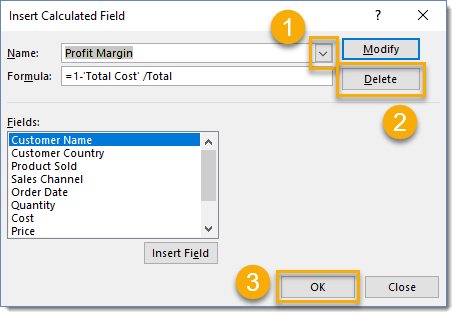
Delete a calculated field from the Insert Calculated Field dialog box.

1. Use the drop down menu to select the calculated field you want to delete.
2. Press the Delete button.
3. Press the OK button.

The calculated field will no longer show up in your PivotTable Field list. Note, this can’t be undone!

Insert a Calculated Field with a Keyboard Shortcut

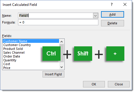
You can quickly open the Insert Calculated Field dialog box to create a new calculated field or edit an existing calculated field by using the Ctrl + Shift + + keyboard shortcut.

Add a Calculated Item

If adding a calculated field is like adding a new column to your source data, then adding a calculated item is like adding a new row.

Let’s say we have a simple table set up that shows the product sold along with the total sales. Our Total column in the data doesn’t include any tax, but there is a 15% chair tax we need to include in our analysis. No problem, we can add this with a Calculated Item!

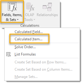
Select a field cell in your pivot table (the calculated item option will be grayed out if you select a value cell). Go to the Analyze tab then press the Fields, Items & Sets button in the Calculations section. Select Calculated Item from the menu.

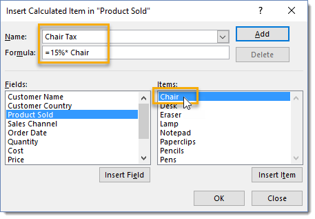
Give your new calculated row a name, then add in a formula. You can add an item into the calculation by selecting the appropriate field then double clicking on any of the items in the field or pressing the Insert Item button.

I named the calculation Chair Tax and the formula will calculate 15% of the value being summarized.

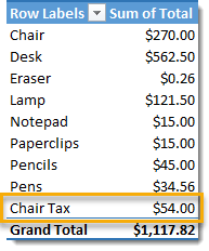
We now see a new row called Chair Tax appear in our Product Sold field and the value is 15% of the Chair value. Note that this new row does contribute to the grand total.

Replace Errors

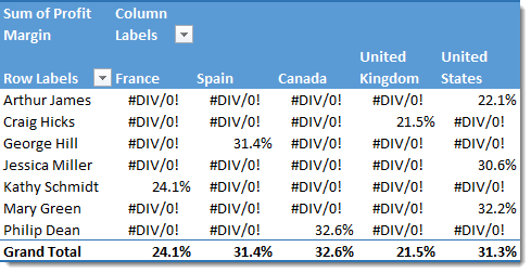
If you create a calculated field with a division operation like our profit margin calculation, then it’s possible you might see some #DIV/0! errors (divide by zero). You can replace these with a number like 0 or some text of your choosing to make the table more presentable. Seeing these errors won’t instill confidence in your audience, so it’s best to replace them with something more assuring.

Select your pivot table and go to the Analyse tab and select Options in the PivotTable section.

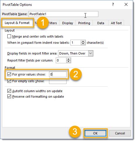
Enable error values option.

1. Go to the Layout & Format tab.
2. Check the For error values show box and input a value or some text.
3. Press the OK button.

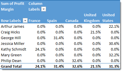
Now your pivot table will be much more presentable.

Add Relationships to Between Tables

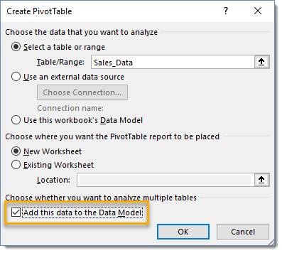
You can create relationships between different data tables using pivot tables and the Data Model. When creating a pivot table check the Add this to the Data Model box in the Create PivotTable window.

For example if our sales data only contained a customer ID and the customers name was stored in another table, this would allow us to relate the customer ID to the name and build sales data pivot tables based on the customer name.

Read this post for more detail on building relationships in pivot tables.

Create a PivotChart

Pivot tables are amazing, but even with a pivot table it’s sometimes hard to see the trend or anomaly in the data. PivotCharts allow you to create a visualization of your pivot table summary.

The cool thing is, they are dynamically linked together. If you change something in your pivot table the changes will happen in your pivot chart and vise-versa.

You can turn your pivot tables into a variety of different chart types.

• Column charts
• Line charts
• Pie charts
• Bar charts
• Area charts
• Radar charts

To insert a PivotChart select the pivot table you want to create PivotChart based on. Go to the Analyze tab in the ribbon and select PivotChart from the Tools section. Select the type of chart you want from the Insert Chart menu.

This can also be accessed from the Insert tab in the Charts section with the PivotChart command.

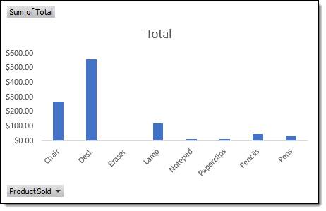
Now we have a visual representation of our pivot table! You can use the field buttons in the chart (lower left corner in the above example) to filter and sort your chart, notice this will also update your pivot table!

Insert a PivotChart with a Keyboard Shortcut

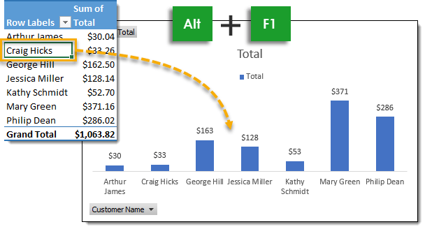
Select a cell inside your pivot table and press Alt + F1 to quickly add a PivotChart to the same sheet as your pivot table.

You can use the alternate ribbon command shortcut keys of Alt + N + SZ

Add a Slicer

Slicers are great for making dynamic and interactive dashboards. They work exactly like a filter but the list of filtered items will remain visible to the user.

Go to the Analyze tab in the ribbon and select Insert Slicer under the Filter section.

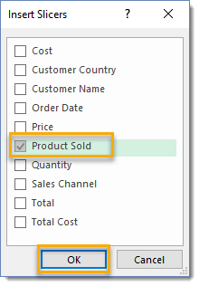
Select the fields for which you want to create the slicer. Selecting multiple fields will result in a separate slicer for each field selected.

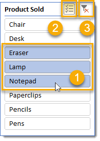
You can now filter on any combination of items from your slicer.

1. Select any item with a left click. You can select multiple adjacent items with a left click and drag.
2. Turn on multi-select mode to select multiple non-adjacent items.
3. Clear your selected filter and start again.

Add a Timeline

To add a Timeline to your pivot table or chart, your source data will need to contain a date field.

Timelines are exactly like Slicers, but only for use with date fields. They allow you to filter on dates with a visual time line slider bar.

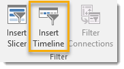
Go to the Analyze tab in the ribbon and select Insert Timeline under the Filter section.

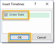
Select the date fields for which you want to create the Timeline. Selecting multiple fields will result in a separate timeline for each field selected.

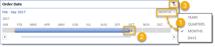
You can now filter your data on any range of dates from your Timeline.

1. Select to filter by Days, Months, Quarters or Years.
2. Drag the end of the timeline to adjust the filtered range. Unfortunately, there is no multi-select like the slicers and you can only select one continuous range of dates.
3. Clear your filter to start again.

Hide All Field Buttons on a Pivot Chart

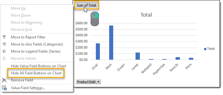
Generally speaking, having less junk on your charts is better! This is why I like to remove all the buttons on a PivotChart to free up valuable chart real estate. Any filtering needed can be done from the linked pivot table instead of from the chart.

Right click on any of the buttons on the chart and select Hide All Field Buttons on Chart.

Connect Slicers or Timelines to Multiple Pivot Tables

You can connect your slicers and timelines to any number of pivot tables. This means you can control many pivot tables or pivot charts from one single slicer or timeline. This is great for creating interactive dashboards.

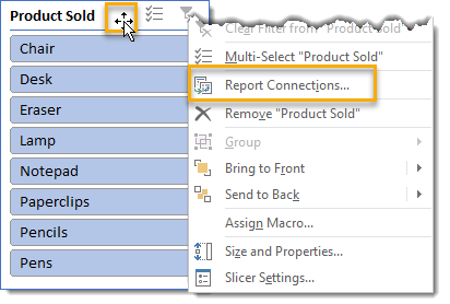
Right click on the slicer or timeline and then select Report Connections from the menu. You can also access this from the Slicer Tools Option ribbon tab when your slicer is selected.

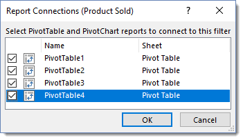
Select any pivot tables you want to connect to the slicer by checking the corresponding box and press the OK button. This is where properly naming your pivot tables can really pay off.

Change the Number of Columns in a Slicer

If your field has a lot of items in it, you can conserve some space while still showing all items in the slicer by adjusting the number of columns.

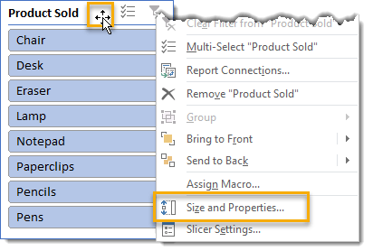
Right click on the slicer and then select Size and Properties from the menu.

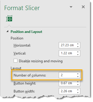
In the Format Slicer window under the Position and Layout section set the desired Number of columns.

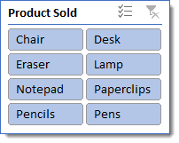
Now you can fit the same number of items in a smaller area within your slicer.

Filter on Top N Items

You can add filters to show your top or bottom N from your pivot table.

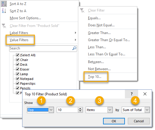
From the filter icon, go to the Value Filters section and select Top 10. You will be able to select from a variety of options.

1. Select to either show the Top or Bottom results from your pivot table.
2. Select a number of items, percentage or total sum for the top or bottom criteria.
3. Select from either Items, Percent or Sum.
   • Items – This will show the items in your field that have the highest or lowest N values.
   • Percent – This will show the items in your field where the value is in the top or bottom Nth percentile.
   • Sum – This will show the top or bottom items in your field where the sum is greater than the number entered in step 2.
4. Select the metric in your pivot table values area to base the top or bottom results on.

Add a Value Filter for any Field

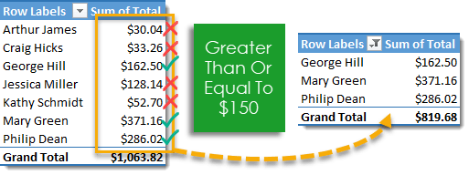
We can filter any field in the row or column area of a pivot table based on the associated value in the values area.

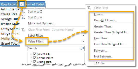
Click on the filter icon to the right of the field name. Select Value Filters from the menu. From here you can select any number of options.

• Filter on items where the value Equals a given value.
• Filter on items where the value Does Not Equal a given value.
• Filter on items Greater Than a given value.
• Filter on items Greater Than Or Equal To a given value.
• Filter on items Less Than a given value.
• Filter on items Less Than Or Equal To a given value.
• Filter on items Between two given values.
• Filter on items Not Between two given values.

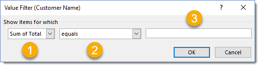
Regardless of which value filter option you selected, you’ll be able to adjust it from the value filters criteria menu.

1. Select which values field your criteria will apply to.
2. Select the filtering option desired. This allows you to change the option you previously selected.
3. Enter the criteria value to filter based on. If you selected a filtering option that requires two inputs, there will be two input fields here.

Increase the Row Label Indent in Compact Form Layout

You can increase the indent for row labels in a compact form layout pivot table to add a bit more of a distinct separation between fields.

Select your pivot table and go to the Analyze tab and select Options.

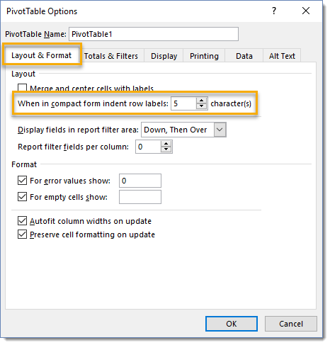
Go to the Layout & Format tab then adjust the character count for your indent as desired.

Add Multiple Subtotal Calculations

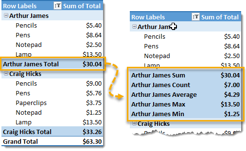
When you add subtotals to your pivot table, by default it will just show the sum subtotal. It is possible to change this to show a different calculation like Count, Average, Minimum, Maximum, Standard Deviation and others. It’s also possible to show multiple different subtotal calculations at the same time!

For this, you’ll need to have a pivot table with at least two fields in the rows area of the pivot table.

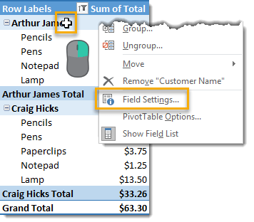
Right click on the field you’re going to add different subtotals to and then select Field Settings from the menu.

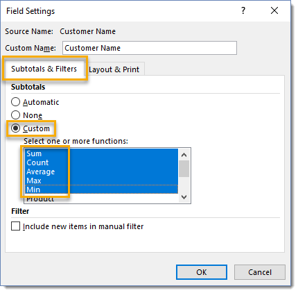
From the Field Settings menu under the Subtotals & Filters tab select the Custom subtotals option then select any Subtotal Calculation type.

This is an awesome way to show more summary information in your pivots.

Include New Items in Manual Filters

Let’s say you’ve spent a decent amount of time manually filtering your pivot table to a select number of field items.

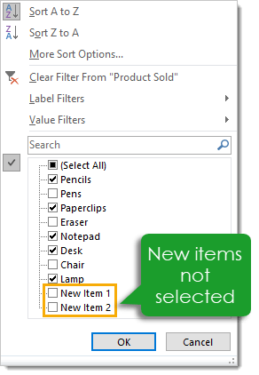
You then add data to your source data set and the new data contains additional items in your field which weren’t in the previous data.

When you refresh your pivot table, the new data items will not be included in the filtered items. You have to go through and manually select those new items if you want them to appear in the filtered pivot table.

You can change this so that new data items in a field are automatically added to any manual filters. Right click on the field then select Field Settings.

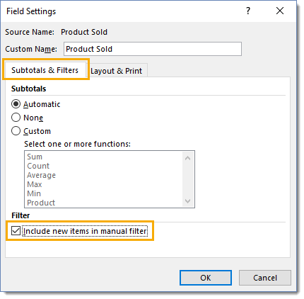
From the Field Settings menu go to the Subtotals & Filters tab and check the Include new items in manual filter box.

Use an External Data Connection Source

You can use an external data source for your pivot table. This means you can store your data in another Excel file or CSV and do your analysis in a separate workbook. Your data can be updated by other people or systems without affecting your current workbook and analysis.

Select the cell where you want your new pivot table to appear then go to the Insert tab in the ribbon and select PivotTable from the Tables section.

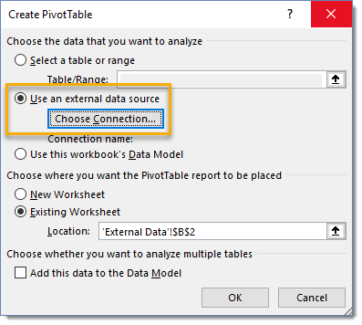
From the Create PivotTable menu select the Use an external data source radio button then click on the Choose Connection button.

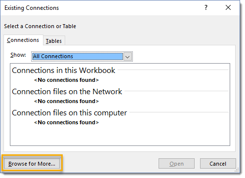
In the Existing Connection menu select Browse for More. In the resulting file picker menu, navigate to the desired file and select it then press the Open button.

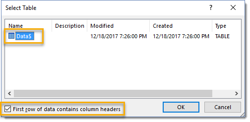
In the resulting select table menu select the location of the data from your file. My data was in a table on a sheet called Data so I have selected Data$ from the list. Make sure to check the First row of data contains column headers box if your data has column headers and then press the Ok button.

You can now finish creating and building your pivot table as usual.

Refresh External Connections on a Schedule

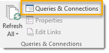
You can set up your external connections to refresh with any new or updated data on a periodic schedule of your choosing. Go to the Data tab in the ribbon and select the Queries & Connections command.

If you select the pivot table with your external connection first, you can directly open the Properties menu from the Data tab.

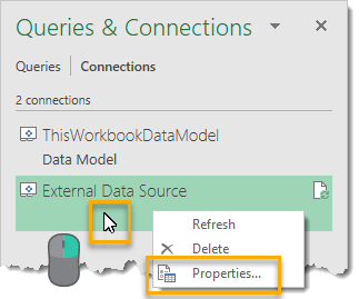
Right click on the external connection from the Queries & Connections window and select Properties from the menu.

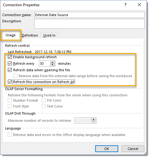
Under the Usage tab in the Connection Properties menu, check the Refresh every N minutes box and then set the number of minutes.

Note that all the Refresh control options are disabled (unchecked) by default. You can also enable a few other options from this menu.

• Enable background refresh
• Enable Refresh data when opening the file
• Enable Refresh this connection on Refresh All

Show Value As

The next 10 tips are the among the most powerful features of pivot tables, yet most Excel users don’t know about them.

At some stage you’ve probably gone off to the side of your pivot table and done some formula calculations to see how much of a percentage a value represents, calculated a running total or a percent difference. This stuff is already a baked in feature known as Show Values As.

Unfortunately it’s sort of hidden in the right click menu or as the secondary tab in the Value Field Settings. It’s so useful and powerful it really deserves a featured spot in the Analyze tab of the ribbon.

You can access this feature a couple of different ways.

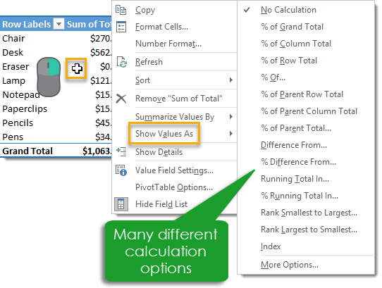
Right click on any value and then select Show Values As from the menu. In the sub-menu you’ll be able to select from many different calculation options. You’ll also be able to set a field back to No Calculation from here.

Another option is to access this through the Value Field Settings menu.

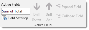
Go to the Analyze tab and press the Field Settings button found under the Active Field section.

Or you can right click anywhere on the field to open the menu and then select Value Field Settings.

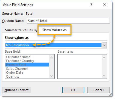
Once you’re at the Value Field Settings menu go to the Show Values As tab.

There are many options here as to how to display your values. We’ll explore these in the following tips.

Show Value as % of Grand Total

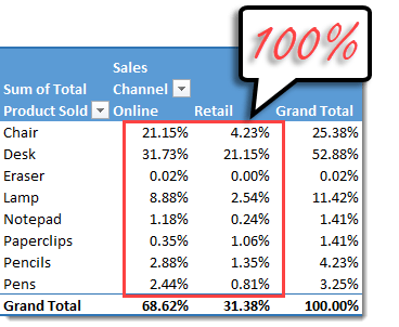
Select the % of Grand Total option to show all values as a percent of the grand total. When selected the Grand Total will show as 100% and all the values in the Value area will add up to 100%.

Show Value as % of Column Total

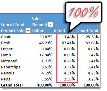
Select the % of Column Total option to show all values in each column as a percent of that columns total. When selected each column total will show as 100% and all the values in each column will add up to 100% including the Grand Total column.

Show Value as % of Row Total

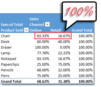
Select the % of Row Total option to show all values in each row as a percent of that rows total. When selected each row total will show as 100% and all the values in each row will add up to 100% including the Grand Total row.

Show Value as % of Parent Column

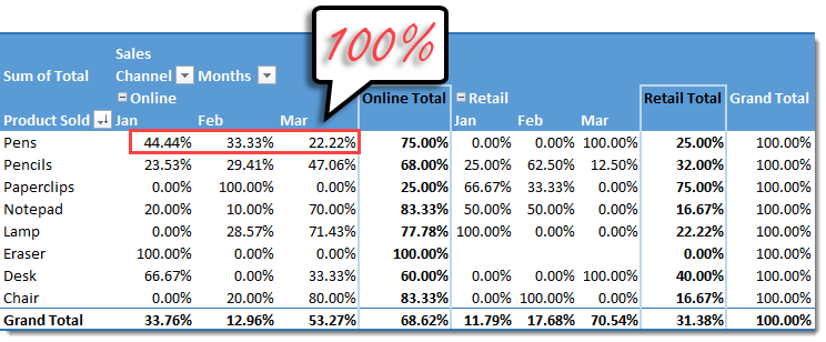
Select the % of Parent Column option to show all values in each row as a percent of its parent column. Each row of values within a parent column will add to 100%. The Grand Total column will contain all 100% values.

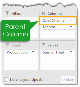
A parent column will be the top most field in the Columns area of the pivot table.

Show Value as % of Parent Row

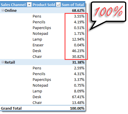
Select the % of Parent Row option to show all values in each column as a percent of its parent row. Each column of values within a parent row will add to 100%. The Grand Total row will contain all 100% values.

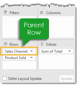
A parent row will be the top most field in the Rows area of the pivot table.

Show Value as Difference

Select the Difference From option to show all values as the difference between the current item and previous item, next item or a fixed item’s value.

Show Value as % of Difference

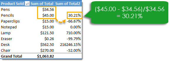
Select the % Difference From option to show all values as the percent difference between the current item and previous item, next item or a fixed item’s value.

Show Value as Running Total

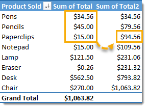
Select the Running Total In option to show a running total for a given field.

Show Value as % of Running Total

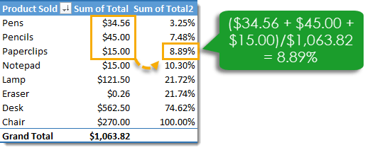
Select the % Running Total In option to show the running total for a given field as a percent of the Grand Total.

Show Value as Rank

Select the Rank Smallest to Largest or Rank Largest to Smallest option to show a fields rank.