
Given a date value in Excel, is it possible to extract the month name?
For example, given the 2020-04-23 can you return the value April?
Yes, of course you can! Excel can do it all.
In this post you’ll learn 8 ways you can get the month name from a date value.
Long Date Format
You can get the month name by formatting your dates!
Good news, this is super easy to do!
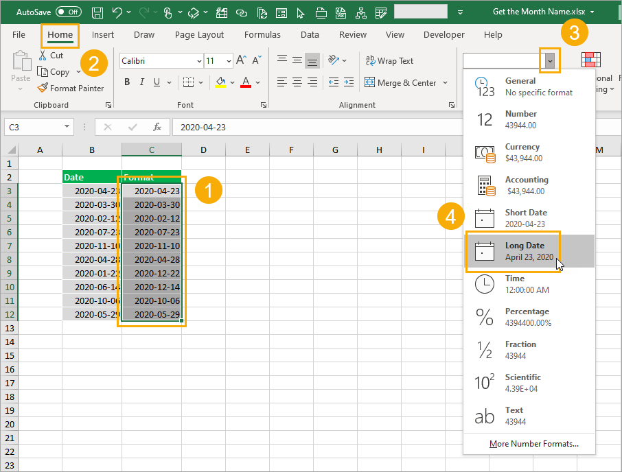
Format your dates:
- Select the dates you want to format.
- Go to the Home tab in the ribbon commands.
- Click on the drop-down in the Numbers section.
- Select the Long Date option from the menu.

This will format the date 2020-04-23 as April 23, 2020, so you’ll be able to see the full English month name.
This doesn’t change the underlying value in the cell. It is still the same date, just formatted differently.
Custom Formats
This method is very similar to the long date format, but will allow you to format the dates to only show the month name and not include any day or year information.

Select the cells you want to format ➜ right click ➜ select Format Cells from the menu. You can also use the Ctrl + 1 keyboard shortcut to format cells.

In the Format Cells dialog box.
- Go to the Number tab.
- Select Custom from the Category options.
- Enter mmmm into the Type input box.
- Press the OK button.

This will format the date 2020-04-23 as April, so you’ll only see the full month name with no day or year part.
Again, this formatting won’t change the underlying value, it will just appear differently in the grid.
You can also use the mmm custom format to produce an abbreviated month name from the date such as Apr instead of April.
Flash Fill
Once you’ve formatted a column of date values in the long date format shown above, you’ll be able extract the name into a text value using flash fill.

Start typing a couple examples of the month name in the adjacent column to the formatted dates.
Excel will guess the pattern and fill its guess in a light grey. You can then press Enter to accept these values.
This way the month names will exist as text values and not just formatted dates.
TEXT Function
The previous formatting methods only changed the appearance of the date to show the month name.
With the TEXT function, you’ll be able to convert the date into a text value.

= TEXT ( B3, "mmmm" )The above formula will take the date value in cell B3 and apply the mmmm custom formatting. The result will be a text value of the month name.
MONTH Functions
Excel has a MONTH function which can extract the month from a date.
MONTH and SWITCH
This is extracted as a numerical value from 1 to 12, so you will also need to convert that number into a name somehow. To do this you can use the SWITCH function.

= SWITCH (
    MONTH(B3),
    1,"January",
    2,"February",
    3,"March",
    4,"April",
    5,"May",
    6,"June",
    7,"July",
    8,"August",
    9,"September",
    10,"October",
    11,"November",
    12,"December"
)
The above formula is going to get the month number from the date in cell B3 using the MONTH function.
The SWITCH function will then convert that number into a name.
MONTH and CHOOSE
There’s an even more simple way to use the MONTH function as Wayne pointed out in the comments.
You can use the CHOOSE function since the month numbers can correspond to the choices of the CHOOSE function.
= CHOOSE (
    MONTH(B3),
    "January",
    "February",
    "March",
    "April",
    "May",
    "June",
    "July",
    "August",
    "September",
    "October",
    "November",
    "December"
)
The above formula is will get the month number from the date in cell B3 using the MONTH function, CHOOSE then returns the corresponding month name based on the number.
Power Query
You can also use power query to transform your dates into names.
First you will need to convert your data into an Excel table.

Then you can select your table and go to the Data tab and use the From Table/Range command.
This will open up the power query editor where you’ll be able to apply various transformation to your data.
Transform the date column to a month name.
- Select the column of dates to transform.
- Go to the Transform tab in the ribbon commands of the power query editor.
- Click on the Date button in the Date & Time Column section.
- Choose Month from the Menu.
- Choose Name of Month from the sub-menu.
This will transform your column of dates into a text value of the full month name.
= Table.TransformColumns ( #"Changed Type", {{"Date", each Date.MonthName(_), type text}} )This will automatically create the above M code formula for you and your dates will have been transformed.
You can then go to the Home tab and press Close & Load to load the transformed data back into a table in the Excel workbook.
Pivot Table Values
If you have dates in your data and you want to summarize your data by month, then pivot tables are the perfect option.

Select your data then go to the Insert tab and click on the Pivot Table command. You can then choose the sheet and cell to add the pivot table into.

Once you have your pivot table created, you will need to add fields into the Rows and Values area in the PivotTable Fields window.
Drag and drop the Date field into the Rows area and the Sales field into the Values area.
This will automatically create a Months field that summarizes the sales by month in you pivot table and the abbreviated month name will appear in your pivot table.
Power Pivot Calculated Column
You can also create calculated columns with pivot tables and the data model.
This will calculate a value for each row of data and create a new field for use in the PivotTable Fields list.

Follow the same steps as above to insert a pivot table.
In the Create Pivot Table dialog box, check the option to Add this data to the Data Model and press the OK button.
After creating the pivot table, go to the Data tab and press the Manage Data Model command to open the power pivot editor.

= FORMAT ( Table1[Date], "mmmm" )Create a new column with the above formula inside the power pivot editor.
Close the editor and your new column will be available for use in the PivotTable Fields list.

This calculated column will show up as a new field inside the PivotTable Fields window and you can use it just like any other field in your data.
Conclusions
That’s 8 easy ways to get the month name from a date in Excel.
If you just want to display the name, then the formatting options might be enough.
Otherwise, you can convert the dates into names with flash fill, formulas, power query or even inside a pivot table.
What is your favourite method?


![6 Ways to Count Colored Cells in Microsoft Excel [Illustrated Guide]](http://cdn-5a6cb102f911c811e474f1cd.closte.com/wp-content/uploads/2021/08/Count-Coloured-Cells-in-Excel.png)


Hi John. Good post. Here’s another using CHOOSE, as in: =CHOOSE(MONTH(B3),”January”,”February”,”March”,”April”,”May”,”June”,”July”,”August”,”September”,”October”,”November”,”December”). Thanks for all the great tips and videos. Thumbs up!!
Thanks Wayne. Much more efficient than using SWITCH. I’ll have to add that one into the post. Thanks.
Cool! Thanks :))
It’s up there now. Thanks!
:))