Do you find it challenging to re-adjust the column width of copied data from an Excel worksheet or table? Did you know you could also copy column width in Excel when copying a cell or cell range?
Excel is a powerful tool that streamlines your data structuring and organization tasks. Sometimes, even the simplest operations can leave you scratching your head. One such common challenge is copying column widths.
If you’ve ever spent valuable time manually adjusting column widths to match across different worksheets or workbooks, worry no more! In this article, we’ll unravel the secret to effortlessly copying column widths in Excel.
Discover handy tips, shortcuts, and techniques to ensure consistent column widths, saving you precious time and annoyance. Whether you’re a beginner or an experienced Excel user, this guide will empower you to conquer this common Excel puzzle with ease and efficiency.
What Is Copying Column Width in Excel?
Copying column width in Excel refers to the process of duplicating the width measurement of one column and applying it to another column. Column width determines the amount of space allotted to display data in a specific column.
When working with large datasets or multiple worksheets, it can be time-consuming to manually adjust column widths to match. By copying column width, you can ensure consistency and uniformity across columns, enhancing the visual appeal and readability of your Excel spreadsheets.
This technique eliminates the need for repetitive resizing and saves valuable time, allowing you to focus on analyzing and manipulating your data effectively.
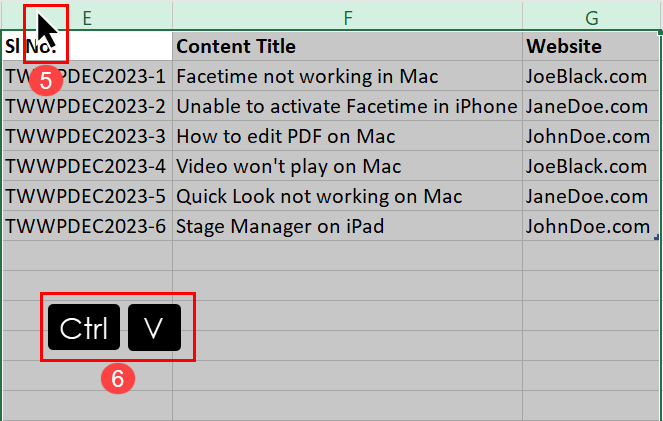
For example, if you copy the following dataset from A1:C7 to E1:G7, you get the following view of the copied data:

The copied content isn’t visible. So, you need to manually adjust the column width by double-clicking the edge of each column header. Or you could drag the column width as well. It might look okay for three columns, but when there are hundreds of columns, it’s a daunting task.
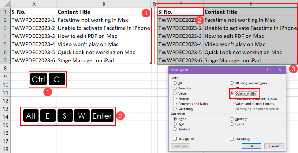
In this situation, you can utilize the tricks explained in this article to automatically match the column width in the destination cell range or worksheet according to the source dataset or table. Here’s an example:

Copy Column Width By Copying the Whole Column
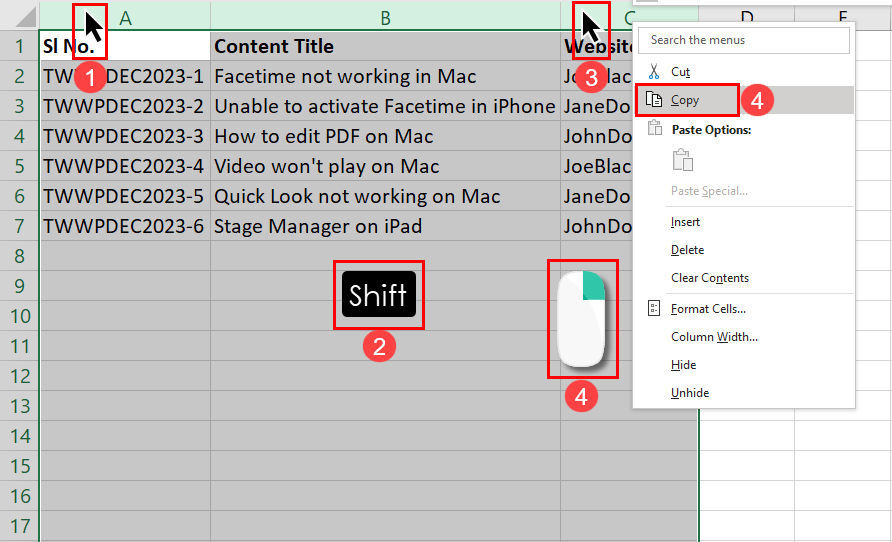
If you need to quickly copy column width from source to target, copy the whole column to the destination worksheet or column on the same worksheet. Here’s how:

- Click the first column header
(A)of the source data. - Press the Shift key.
- Click the last column header
(C)of the source data. - Right-click and select Copy on the context menu.

- Select the first column header
(E)of the destination. - Press Ctrl + V to copy the data as well as the column width.
Use the Format Painter Tool to Copy Column Width in Excel
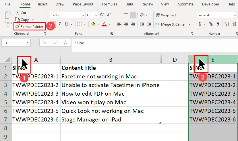
Another simple way to apply the column width of the source column in the destination column is by using the Format Painter tool in Excel. Here is how you can also do it:

- Select the column header
(A)of the source. - Click the Format Painter tool inside the Clipboard block of the Home tab.
- Now, click the column header
(E)of the target column. - Excel will copy the column width and apply that to the target column.
Copy Column Width in Excel Using Paste Special
The Paste Special tool of Excel offers various modes of copying and pasting data. One such mode is copying data along with the source column widths. Here are the steps to learn this method:

- Select the cell range of a dataset or table you want to copy to another worksheet or the cell range of the same worksheet.
- Hit the Ctrl + C keys to copy the data to the clipboard.
- Highlight the first cell of the destination cell range or worksheet.
- Right-click and hover the mouse cursor over the Paste Special option.
- Under the Paste block, click the sixth paste option that says Keep Source Column Widths.

- You should get the copied data in the destination cell range along with the source column widths.
Use A Shortcut to Copy Column Width in Excel
Suppose you already copied the data to the destination. Now, you’d like to apply the source column widths as well. In this case, you can use a series of keyboard keys instead of clicking the Excel user interface. Here’s how:

- Select the cell range of source data and press Ctrl + C to copy it.
- Now, highlight the first cell of the target cell address and press the following keys in the given order:
Alt > E > S > W > Enter
- Excel will format the target dataset by copying the column widths from the source dataset.
Copy Column Width in Excel Using Excel VBA
The methods mentioned so far, though copy the column’s widths automatically, still need to press a few keys. So, you must remember those keys if you want to apply the source dataset columns widths to the destination worksheet or cell range.
Also, you can’t really integrate this as an automated workflow when you use Excel VBA to automate the rest of the data organization process. In such a scenario, you need a VBA script to export the source column width to a new destination where you’re copying data.
You could use the following two VBA scripts:
Just Copy Column Width
You can use this code to apply a source column width to a target column. For example, you copied the data from A1:C7 to E1:G7. Now, you want to apply the column width of column A to column E only not for all other columns. In this scenario, follow these steps and use the following VBA script:

- Hit Alt + F11 to bring up the Excel VBA Editor on the worksheet you’re working on.
- Now, click the Insert button on the VBA Editor toolbar and select Module.
- This will create a blank module where you need to copy and paste the following VBA script:
Sub CopyColumnWidth()
    Dim sourceColumn As Range
    Dim targetColumn As Range

    ' Set the source column
    Set sourceColumn = Range("A:A") ' Replace "A:A" with the desired source column

    ' Set the target column
    Set targetColumn = Range("E:E") ' Replace "E:E" with the desired target column

    ' Copy the column width
    targetColumn.ColumnWidth = sourceColumn.ColumnWidth
End Sub
- In the above VBA code, ensure you customize the following if the source and target cell ranges are different than the data shown in this tutorial:
Range("A:A")represents the column width of the source column, so change the range according to your worksheet.Range("E:E")is the destination column whose width you want to adjust according to the source column. So, change this as well.
- Once done modifying the code, click the Save button and close the VBA Editor tool.

- Hit Alt + F8 to bring up the Macro dialog box and select CopyColumnWidth() macro.
- Click the Run button.
- Excel should automatically fix the column width of the destination column.
Copy Column Width and Data
If you want to automatically copy the dataset from one cell range to another and keep the column width of the source data range, try this VBA code instead:
Sub CopyDataWithColumnWidths()
    Dim sourceRange As Range
    Dim targetRange As Range
    Dim sourceColumns As Range
    Dim targetColumns As Range
    Dim i As Long

    ' Set the source range
    Set sourceRange = Range("A1:C7")

    ' Set the target range
    Set targetRange = Range("E1:G7")

    ' Copy the data
    sourceRange.Copy Destination:=targetRange

    ' Set the source columns
    Set sourceColumns = Range("A:C") ' Replace "A:C" with the desired source columns

    ' Set the target columns
    Set targetColumns = Range("E:G") ' Replace "E:G" with the desired target columns

    ' Copy the column widths
    For i = 1 To sourceColumns.Columns.Count
        targetColumns.Columns(i).ColumnWidth = sourceColumns.Columns(i).ColumnWidth
    Next i
End Sub
The above code will automatically copy the dataset available in the cell range A1:C7 to E1:G7. Also, the code will copy the column width of the source columns to the destination columns.
It’s likely that the dataset you want to copy isn’t in the above-mentioned cell range. Also, you may want to copy your data to a different cell range than the one shown above.
So, modify the following code elements according to your own Excel worksheet and requirements:
Range("A1:C7")should be the address range of the data you’re about to copy.Range("E1:G7")is where you want to copy the source data. So, modify this as well.Range("A:C")should be the range of the source columns. If you’re copying data fromB10:D20, the column range should beRange("B:D").Range("E:G")is the column range of the destination cell range. Hence, you must modify this too if you’re not copying data between the column E and G.
When the code is ready, follow the method mentioned earlier to create a module and paste the code there. Then save the script and execute it from the Macro dialog box.
Copy Column Width in Excel Using Office Scripts
Since you’re unable to use the Excel VBA method to automate the copy column width task in Excel on the web app, I introduce another method based on Office Scripts.
Office Scripts lets you automate various actions on Excel desktop and web apps with better options than Excel VBA.
However, this feature is only available to you when you get Microsoft 365 Business Standard and a better subscription. If you see the Automate tab on your Excel desktop or web app, you can use Office Scripts.
Find below the steps to automate the current challenge using this Excel feature:

- Click the Automate tab on the Excel desktop or web app.
- Select the New Script option inside the Scripting Tools block.
- The Office Scripts Code Editor will show up on the right side.
- Click inside the code editor panel and hit Ctrl + A to select all the codes.
- Hit the Delete key to erase the existing codes.

- Now, copy and paste the following code inside the Code Editor panel:
function main(workbook: ExcelScript.Workbook) {
	let selectedSheet = workbook.getActiveWorksheet();
	// Paste to range D1 on selectedSheet from range A1:B7 on selectedSheet
	selectedSheet.getRange("D1").copyFrom(selectedSheet.getRange("A1:B7"), ExcelScript.RangeCopyType.all, false, false);
	// Paste to range D:E on selectedSheet from range A:B on selectedSheet
	selectedSheet.getRange("D:E").copyFrom(selectedSheet.getRange("A:B"), ExcelScript.RangeCopyType.formats, false, false);
}- Click the Save script button to reuse the code in the future.
- Hit the Run button to execute the code.

Excel will automatically copy the values from the cell range A1:B7 to D1:E7 and apply the column widths from columns A and B to columns D and E.
In the above code, you need to modify the following code elements if your current worksheet data isn’t organized as in the above example:
range D1: the first cell of the first column of the destinationrange A1:B7: the range of the source data and column widthsgetRange("D1"):D1to any cell address which will be the first cell of the destinationgetRange("A1:B7"):A1:B7to any cell range that represents the source data and column widthgetRange("D:E"): destination columns where source column widths will be applied; change accordinglygetRange("A:B"): the source columns to copy column widths; change it according to your dataset
Conclusions
Structuring and organizing data in Excel shouldn’t be complicated or time-consuming. All you need to do is know the tricks to easily restructure copied data like the ones mentioned above.
Here, you learned several methods to copy the column width to the destination worksheet from the source worksheet or an Excel table.
Use the one that suits your needs and comment below to share your experience of using the above tricks in Excel. If you also know a better way to accomplish the same, don’t hesitate to comment.
 👉 Find out more about our Advanced Formulas course!


0 Comments