Do you want to make a table in Excel? This post is going to show you how to create a table from your Excel data.

Entering and storing data is a common task in Excel. If this is something you’re doing, then you need to use a table.

Tables are containers for your data! They help you keep all your related data together and organized.

Tables have a lot of great features and work well with other tools inside and outside of Excel, so you should definitely be using them with your data.

This post is going to show you all the ways you can create a table from your data in Excel. Get your copy of the example workbook used in this post and follow along!

Tabular Data Format for Excel Tables

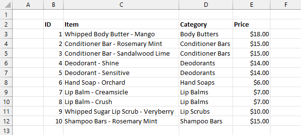
Excel tables are the perfect container for tabular datasets due to their row and column structure. Just make sure your data follows these rules.

• The first row of your dataset should contain a descriptive column heading.
• Your data should have no blank column headings.
• Your data should have no blank columns or blank rows.
• Your data should have no subtotals or grand totals.
• One row in your data should represent exactly one record of data.
• One column should contain exactly one type of data.

If your data is rectangular in shape and adheres to the above rules, then it’s ready to be put into a table.

Create a Table from the Insert Tab

Now that your data is ready to be placed inside a table, how can you do that?

It’s very easy and will only take a few clicks!

You’ll be able to add your data in a table from the Insert tab. Follow these steps to get your data into a table!

1. Select a cell inside your data.
2. Go to the Insert tab.
3. Select the Table command in the Tables section.

This is going to open the Create Table menu with your data range selected. You should see a green dash line around your selected data and you can adjust the selection if needed.

4. Check the My table has headers option. This is needed if the first row of your data contains column name headings.
5. Press the OK button.

Your data is now inside a table! You’ll easily be able to tell the data is inside an Excel Table now because a default table formatting is automatically applied.

You can go to the Table Design tab and select other style options from the Table Styles section.

💡 Tip: Your table will get a default name such as Table1. You should give your new table a descriptive name as this is how you will refer to it in formulas and other tools.

Create a Table from the Home Tab

Another place you can access the table command is from the Home tab.

You can use the Format as Table command to create a table.

1. Select a cell inside your data.
2. Go to the Home tab.
3. Select the Format as Table command in the Styles section.

4. Select a style option for your table.
5. Check the option for My table has headers.
6. Press the OK button.

This is a great option as you get to choose the table style during the process of making your table.

Create a Table with a Keyboard Shortcut

Creating a table is such a common task that there is a keyboard shortcut for it.

Select your data and press Ctrl + T on your keyboard to turn your dataset into a table.

This is an easy shortcut to remember since T stands for Table.

There is also a legacy shortcut available from when tables were called lists. Select your data and if you press Ctrl + L this will also make a table. In this case, L stands for List.

Create a Table with Quick Analysis

When you select any range Excel will show you the Quick Analysis options in the lower right corner.

This will give you quick access to conditional formatting, pivot tables, charts, totals, and sparklines. The menu also includes the table command to convert the data into a table.

You can follow these steps to create a table from the Quick Analysis tools.

1. Select your entire dataset. You can select any cell in the data and press Ctrl + A and this will select the full range.

This should automatically show the Quick Analysis tool in the lower right corner of the selected range.

• Click on the Quick Analysis tools or press Ctrl + Q to open the Quick Analysis menu.
• Go to the Tables tab.
• Click on the Table command. When you hover your cursor over the Table command it will show you a preview of your data inside a table!

📝 Note: This method allows you to skip the Create Table menu and the Quick Analysis will guess if your data has column headings or not. Excel will apply any column headings to your table accordingly.

Quick Analysis can be disabled from the Excel Options menu if the pop-up command is something you find annoying.

1. Go to the File tab.
2. Select the Options menu.
3. Go to the General tab of the Excel Options menu.
4. Uncheck the Show Quick Analysis options on selection option.
5. Press the OK button.

📝 Note: This will only disable the small pop-up command from showing when you select your data. You can still use the Ctrl + Q keyboard shortcut to access the Quick Analysis tools for any selected range.

Create a Table with Power Query

Power Query is a very useful tool for transforming your data, but you can also create a table during the process of building your queries.

If your data isn’t already inside a table, you can use the From Table/Range query to make a table.

1. Select your data.
2. Go to the Data tab.
3. Press the From Table/Range command in the Get & Transform Data section.

This will open the Create Table menu.

4. Check the My table has headers option if the first row in your data contains column headings.
5. Press the OK button.

This will add your data to a table and then open the Power Query Editor where you will be able to build your query based on the new table.

When you are finished building your query, you can go to the Home tab of the Power Query editor and press the Close and Load command.

This will give you the option to create another table filled with the transformed data. Select the Table option and press the OK button to load the transformed data into a table.

⚠️ Warning: This method does create a table, but doesn’t give you the opportunity to name the table before you build your queries. This means your queries will reference the generic table name such as Table1, and if you later change the table name you will also have to update the reference in your query.

Create Multiple Tables from a List with VBA

Suppose you need to create multiple tables in your Excel file. Maybe you need to create a table of sales data for each month of the year. Doing this manually could be a time-consuming process.

This is where you could use VBA to create multiple tables with the required columns.

Go to the Developer tab and select the Visual Basic command to open the visual basic editor. Then go to the Insert tab of the visual basic editor and select the Module option to create a new module to add your VBA macro.

Sub AddTables()
Dim myRange As Range
Dim sheetTest As Boolean
Dim myHeadings As Variant
Dim colCount As Integer
Set myRange = Selection

myHeadings = [{"ID","Date","Item","Quantity","Price"}]
colCount = UBound(myHeadings)

For Each c In myRange.Cells
sheetTest = False
    For Each ws In ThisWorkbook.Worksheets
        If ws.Name = c.Value Or c.Value = "" Then
            sheetTest = True
        End If
    Next ws
    If Not (sheetTest) Then
        With Sheets
            Sheets.Add.Name = c.Value
            Sheets(c.Value).Select
            Range("A1").Resize(1, colCount).Value = myHeadings
            ActiveSheet.ListObjects.Add(xlSrcRange, Range("A1").Resize(1, colCount), , xlYes).Name = c.Value & "Sales"
        End With
    End If
Next c
End Sub

This code will loop through the selected range and add a new sheet for each cell in the range. The code tests if the sheet name exists and if it doesn’t then it creates a new sheet named from the cell value.

The column headings are added to the new sheet starting at cell A1. This is then turned into a table and the table is named based on the sheet name.

myHeadings = [{"ID","Date","Item","Quantity","Price"}]

The above line of code is used to create the column headings in each table. You can adjust this to suit your needs.

You can then run this macro to create multiple tables.

1. Select the range of cells that contain the list the names for each table you want to create. For example, you might want a list of month names to create a table for each month.
2. Press the Alt + F8 keyboard shortcut to open the Macro menu.
3. Select your macro.
4. Press the Run button.

This will run and create a new sheet for each item in your selection. Each sheet will contain a table with the same column headings and be named based on the items in the selected list.

Create Multiple Tables from a List with Office Scripts

If you are using Excel online and want to automate the process of creating multiple tables from a list, then you will need to use Office Scripts.

This is a JavaScript based language that can help you automate tasks in Excel online.

Go to the Automate tab and select the New Script command to open the Office Script Editor.

function main(workbook: ExcelScript.Workbook) {

	//Create an array with the column headings
	let myHeaders = [["ID", "Date", "Item", "Quantity", "Price"]]
	let colCount = myHeaders[0].length;
	//Create an array with the values from the selected range
	let selectedRange = workbook.getSelectedRange();
	let selectedValues = selectedRange.getValues();
	//Get dimensions of selected range
	let rowHeight = selectedRange.getRowCount();
	let colWidth = selectedRange.getColumnCount();

	//Loop through each item in the selected range
	for (let i = 0; i < rowHeight; i++) {
		for (let j = 0; j < colWidth; j++) {
			try {
				//Create a new sheet with name from the selected range
				let thisSheet = workbook.addWorksheet(selectedValues[i][j]);
				//Add column headings to new sheet and convert to table
				thisSheet.getRange("A1").getAbsoluteResizedRange(1, colCount).setValues(myHeaders);
				let newTable = workbook.addTable(thisSheet.getRange("A1").getAbsoluteResizedRange(1, colCount), true);
				newTable.setName(selectedValues[i][j] + "Sales");
			}
			catch (e) {
				//do nothing
			};
		};
	};
};

Copy and paste the above code into the Code Editor. Press the Save script button to save the script and then you can use the Run button to execute the script.

This Office Script code will loop through the active range in your workbook and create a new sheet for each cell in the selected range and name it based on the value in the cell.

let myHeaders = [["ID", "Date", "Item", "Quantity", "Price"]]

The column headings are added to each new sheet starting in cell A1. You can adjust the above line of code to change the column headings to suit your needs.

These column headings are then turned into a table and the table is named based on the sheet name.

You can then run this script using the following steps.

1. Select a range of cells that contain the list of tables you want to create.
2. Click on the Run button in the Code Editor.

The code will run and create all the sheets with tables in each sheet.

Conclusions

Tables are a very useful feature for your tabular data in Excel.

Your data can be added to a table in several ways such as from the Insert tab, from the Home tab, with a keyboard shortcut, or using the Quick Analysis tools.

Tables work well with other tools in Excel such as Power Query. Because of this, Excel will even automatically convert your data into a table before using Power Query.

Creating multiple tables in your workbook can also be automated using either VBA or Office Scripts.

How do you make your tables? Do you know any other tips? Let me know in the comments section below!