Have you ever wanted to keep a row or column fixed in view while scrolling through your data? This post is going to show you how to freeze rows or columns so they always stay visible.
You will often need to scroll down or to the right to view a particular record or field in a large dataset. But when you scroll too far, you will lose track of the row and column headings!
When working with large datasets, you can use the Freeze Panes feature to ensure the top rows or first few columns will remain visible no matter where you scroll in your sheet.
Follow along to find out how you can freeze the top rows or columns in your Excel sheets!
Freeze Rows and Columns from the Home Tab

The above example shows a large dataset in Excel. Normally when you scroll down or to the right you can see the columns headings and row headings disappear from view.
This makes it hard to tell which record or field you’re looking at.
The Freeze Panes feature will allow you to pin the top row and first column so when you scroll around the sheet they always remain in view. This makes it easy to tell which record or field you’re looking at!
With the Freeze Panes feature, you can customize exactly how many rows or columns you want to keep in view.
Rows and columns can be frozen independently, so you can freeze just the top row, just the first column, or both. You can also freeze more than one row or more than one column. It’s very flexible!
Freeze Only the First Row

Follow these steps to freeze only the top row in your sheet.
- Go to the View tab.
- Click on the Freeze Panes option found in the Window section of the ribbon.

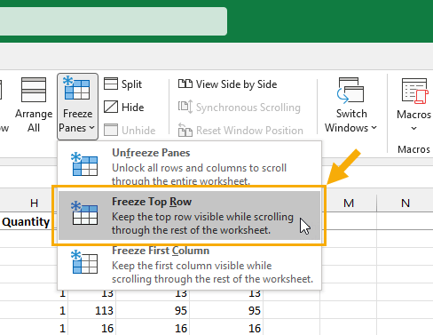
- Choose the Freeze Top Row option from the menu.
This will freeze only the top row in your sheet. When you scroll down, row 1 remains fixed in view!

There is a slight visual indicator to show the top row has been frozen. You will see a slightly darker gray line under the first row.
Freeze Multiple Rows
You can also freeze more than one row to the top, but to do this you will need to make a selection in the sheet first.

Follow these steps to freeze more than one row to the top.
- Select a cell in the first column directly below the rows you want to freeze.
- Go to the View tab.
- Click on the Freeze Panes command.
- Choose the Freeze Panes option from the menu.
In the above example, cell A4 is selected, which means rows 1:3 will be frozen in place.
Freeze Only the First Column

Follow these steps to freeze only the first row in your sheet.
- Go to the View tab.
- Click on the Freeze Panes command in the Window section.
- Choose the Freeze First Column option from the menu.
This will result in Column A getting locked in view when you scroll to the right of the sheet.
Freeze Multiple Columns
You can also freeze mulitple columns at the left of the sheet, but to do this you will need to make a selection in the sheet first.

Follow these steps to freeze more than one column on the left.
- Select a cell in the first row directly to the right of the columns you want to freeze.
- Go to the View tab.
- Click on the Freeze Panes command in the Windows section of the ribbon.
- Choose the Freeze Panes option from the menu.
In this example, cell C1 is selected which means that columns A:B will stay fixed and visible on the left side of the sheet when scrolling.
Freeze Both Rows and Columns
Many times you will want to freeze both rows and columns when you scroll. This is possible with the Freeze Panes option but what rows and columns are frozen will depend on where the active cell is when you use the command.

Follow these steps to freeze any number of rows of columns in your sheet.
- Select a cell directly below and to the right of the rows and columns you want to freeze.
- Go to the View tab.
- Click on the Freeze Panes command in the Windows section of the ribbon.
- Choose the Freeze Panes option from the menu.
In this example, cell C4 is selected which means rows 1:3 and columns A:B will be frozen and stay anchored at the top and to the left of the sheet.
💡 Tip: Select cell B2 before using the Freeze Panes command if you only want to freeze the first row and first column.
Freeze Rows and Columns with a Keyboard Shortcut

There is no dedicated keyboard shortcut for freezing panes in Excel, but you can access the commands with the Alt hotkeys.
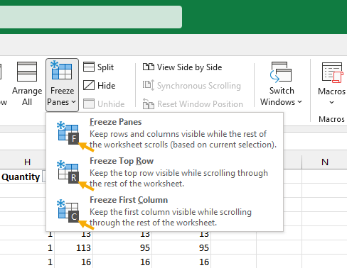
Press the sequence Alt, W, F and this will open the Freeze Panes menu in the View tab. Then you can use the following keys.
- Press the F key to Freeze Panes. This acts as a toggle and will also unfreeze the rows or columns if they are already frozen.
- Press the R key to Freeze Top Row.
- Press the C key to Freeze First Column.
When using the Freeze Panes shortcut, remember to select the cell directly below and to the right of the rows and columns you want to be frozen.
📝 Note: When using the Freeze Panes shortcut, remember to select the cell directly below and to the right of the rows and columns you want to be frozen.
Freeze Top Row with a Table
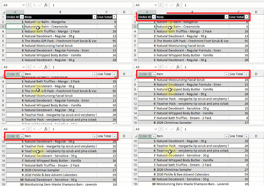
One of the many benefits of placing your data inside an Excel Table object is that when you scroll down the page the column heading will automatically remain pinned to the top when the table is selected.

You can place your data inside an Excel table by following these steps.
- Select any cell inside your data.
- Go to the Insert tab.
- Select the Table command.

- Make sure the selected range contains all your data. You can adjust this range if needed by clicking on the selection button to the right of the range input.

- Check the My table has headers option.
- Press the OK button.
It’s essential that you enable the header option in the Create Table menu. This ensures the first row of your dataset is used in the table column headings and this is what will be pinned to the top when you scroll.

Your data will now be inside a Table. When you scroll down notice the column letters get replaced with the column labels from the table!
📝 Note: Tables will only pin the column headers when you scroll down and won’t pin the first column when you scroll right.
Freeze Rows and Columns with Split Pane
There is another Excel feature that works similarly to Freeze Panes and will allow you to keep the top rows and rightmost columns always visible.
You can use the Split Pane feature to split the sheet into 4 separately scrollable areas. Usually, this is used to simultaneously view up to 4 different disjointed areas in the same sheet.

Follow these steps to keep the first row and first column visible using Split Pane.
- Select cell B2 in the sheet.
- Go to the View tab.
- Click on the Split command in the Window section of the ribbon.

This will put thick gray bars that separate the first row and first column from the rest of the sheet. When you place your cursor in the lower right quadrant and scroll, the top row and first column stay visible!

The best part about using Split Panes instead of Freeze Panes is that it’s very easy to adjust how many rows or columns you want to see.
Hover the mouse cursor over the split pane and the cursor will change to a four-way array. You can then click and drag the split panes to change how many rows and columns stay in view.
💡 Tip: Double left click at the intersection of the split panes to remove them entirely from the sheet.
Freeze Panes with VBA
Using the Freeze Panes feature is easy when you’re working with a single sheet. But if you have many similar sheets on which you want to freeze the top row and first column it can be a tedious task!
You would need to select each sheet, then select cell B2 within, then turn on the Freeze Panes feature. That could be a lot of clicks.
This is definitely a task that can be automated with the use of VBA!

Go to the Developer tab and click on the Visual Basic option to open the visual basic editor. Go to the Insert menu in the editor and select the Module option.
Sub FreezePanesAllSheets()
Dim ws As Worksheet
For Each ws In ThisWorkbook.Worksheets
    ws.Activate
    Range("B2").Select
    ActiveWindow.FreezePanes = True
Next ws
End Sub
Copy and paste the above code into the new module in the editor.
When you run this VBA code it will look through all the sheets in the workbook, then select cell B2 and turn on the Freeze Panes option.
This will make quick work of freezing the first row and first column across your entire workbook!
Freeze Panes with Office Scripts
If you are using Excel online with a Microsoft 365 business plan, then you will be able to automate your tasks with Office Scripts.
This is a JavaScript based language currently only available in the web version of Excel.
You can use Office Scripts to quickly loop through all your sheets and freeze panes in them.

function main(workbook: ExcelScript.Workbook) {
	let sheets = workbook.getWorksheets();

	for (let sheet of sheets) {
			sheet.getFreezePanes().freezeAt("A1");
	};
}
Go to the Automate tab and click on the New Script command. This will open up the Code Editor and you can copy and paste the above code into it.
Press the Save script button and then press the Run button.
The code will turn the freeze panes option on across all the sheets in the workbook.
⚠️ Warning: When you Freeze Panes from the user interface, you need to select the cell directly below and to the right of the rows and columns to freeze. But this works differently in the Office Scripts code. The freezeAt("A1") method requires the selection to be on the last row and column to freeze!
Conclusions
When working with a large dataset in Excel scrolling around will result in hidden row and column headings. This can make it difficult to tell what the data is.
This problem can be easily fixed by using the Freeze Panes feature to fix any number of rows or columns to always be visible.
Freeze Panes can also be activated with either VBA or Office Scripts. This can save you from manually enabling Freeze Panes across all your sheets.
Excel also comes with a useful feature called Split Panes, which allows you to split the sheet into 4 scrollable areas. This can be used to keep rows and columns in view while scrolling through your sheet.
Excel Tables can be an easy alternative to freezing panes. When scrolling down a table, they will always display the column headings at the top.
Do ever freeze rows and columns in your Excel sheets? Do you know any other useful tips to get this done? Let me know in the comments below!
 👉 Find out more about our Advanced Formulas course!


0 Comments