You’re likely going to come across the need for running totals if you’re dealing with any sort of daily data.
Imagine you track sales each day. Your data contains a row for each date with a total sales amount, but maybe you want to know the total sales for the month at each day. This is a running total, it’s the sum of all sales up to and including the current days sales.
In this post we’ll cover multiple ways to calculate a running total for your daily data. We’ll explore how to use worksheet formulas, pivot tables, power pivot with DAX and power query.
We’ll also explore what happens to the running total calculation when inserting or deleting rows of data and how to update the results.
Get the file with all the examples.
Running Totals with a Simple Formula
It’s possible to create a basic running total formula using the + operator.
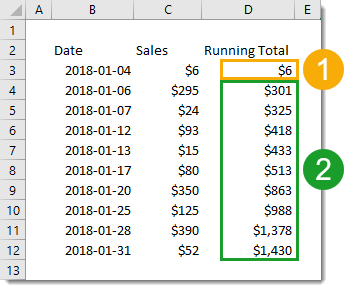
However, we’ll need to use two different formulas to get the job done.
- =C3 will be the first formula and will only be in the first row of the running total.
- =C4+D3 will be in the second row and can be copied down the remaining rows for the running total.
The formula in our first row can’t add the cell above it to the total as it contains a text value for a column heading. This would cause a #VALUE! error to appear in the running total since the + can’t handle text values. We avoid this with a different formula in the first row which doesn’t reference the cell above.
What happens to the running total when we insert or delete rows in our data?
![]()
Inserting a new row will result in a gap in the running total. To fix this, we’ll need to copy the formula down from the first cell above the newly inserted rows all the way down to the last row.

Deleting any rows will result in #REF! errors since deleting a row means deleting a cell referenced by the formula below it. To fix this, we’ll need to copy the formula down from the last error-free cell all the way down to the last row.
Running Totals with a SUM Formula

We can avoid the awkwardness of using two different formulas in our running total column by utilizing the SUM function instead of the + operator. When the SUM function encounters a text cell it will treat it the same as a though it contained a 0.
This way we can use the following formula uniformly for every row including the first row.
=SUM(C3,D2)
This formula will reference the column heading containing text for the first row, but this ok as it’s treated like a 0.
When inserting or deleting rows, we will still encounter the same problems with blank cells and errors. We can fix them the same way as with running totals in the simple formula method.
Running Totals with a Partially Fixed Range
Another option with the SUM function is to only reference the Sales column and use a partially fixed range reference.

If we use the following formula =SUM($C$3:C3), we can copy and paste this down the range. It won’t reference any column headings and the range referenced will grow to each row.
Unfortunately, this too will have the same problems (and solutions) with inserting or deleting rows.
Running Totals with a Relative Named Range
We can avoid the problems with inserting and deleting rows from our data if we use a relative named range. This will refer to the cell directly above no matter how many rows we insert or delete.
This is a trick that involves temporarily switching the Excel reference style from A1 to R1C1. Then defining a named range using the R1C1 notation. Then switching the reference style back to A1.
In R1C1 reference style, cells are referred to by how far away they are from the cell using the reference. For example, =R[-2]C[3] refers to the cell 2 up and 3 to the right of the cell using this formula.
We can use this relative referencing to create a named range that’s always one cell above the referring cell with the formula =R[-1]C.

To switch reference style, go to the File tab then choose Options. Go to the Formula section in the Excel Options menu and check the R1C1 reference style box and then press the OK button.

Now we can add our named range. Go to the Formula tab of the Excel ribbon and choose the Define Name command.

Insert a name like “Above” as the name of the range. Add the formula =R[-1]C into the Refers to input and press the OK button.
We can now switch Excel back to the default reference style. Go to the File tab > Options the Formula section > uncheck the R1C1 reference style box > then press the OK button.

Now we can use the formula =SUM([@Sales],Above) in our running total column.
The named range Above will always refer to the cell directly above. When we insert or delete rows, the relative named range will adjust accordingly and no action is needed.
In fact if we place our data in an Excel Table then the formula will automatically fill down for any new rows since the formula is uniform for the entire column. No action is needed to copy down any formulas.
Running Totals with a Pivot Table

Pivot tables are super useful for summarizing any type of data. There’s more to them than just adding, counting and finding averages. There are many other types of calculations built in, and there is actually a running total calculation!

First, we need to insert a pivot table based on the data. Select a cell inside the data and go to the Insert tab and choose the PivotTable command. Then go through the Create PivotTable window to choose where you want the pivot table, either in a new worksheet or somewhere in an existing one.

Add the Date field into the Rows area of the pivot table, then add the Sales field into the Values area of the pivot table. Now add another instance of the Sales field into the Rows area.
We should now have two identical Sales fields with one of them being labelled Sum of Sales2. We can rename this label anytime by simply typing over it with something like Running Total.
Right click on any of the values in the Sum of Sales2 field and select Show Value As then choose Running Total In.

We want to show the running total by date, so in the next window we need to select Date as the Base Field.
That’s it, we now have a new calculation which displays the running total of our sales inside the pivot table.

What happens if we add or delete a row in our source data, how does this affect the running total? The pivot table calculations are dynamic and will take any new data into account in its running total calculation, we will just need to refresh the pivot table.
Right click anywhere inside the pivot table and choose Refresh from the menu.
Running Totals with Power Pivot and DAX Measures
The first couple steps for this are the exact same using a regular pivot table.
Select a cell inside the data and go to the Insert tab and choose the PivotTable command.

When you come to the Create PivotTable menu, check the Add this data to the Data Model box to add the data to the data model and enable it for use with power pivot.

Place the Date field in the Rows area and the Sales field in the Values area of the pivot table.
With power pivot, we will need to create any extra calculations we want using the DAX language. Right click on the table name in the PivotTable Fields window, then select Add Measure to create a new calculation. Note, this is only available with the data model.

=CALCULATE (
    SUM ( Sales[Sales] ),
    FILTER (
        ALL (Sales[Date] ),
        Sales[Date] <= MAX (Sales[Date])
    )
)
Now we can create our new running total measure.
- In the Measure window, we need to add a Measure Name. In this case we can name the new measure as Running Total.
- We also need to add the above formula into the Formula box.
- The cool thing about power pivot is the ability to assign a number format to a measure. We can choose the Currency format for our measure. Whenever we use this measure in a pivot table the format will automatically be applied.
Press the OK button and the new measure will be created.

There will be a new field listed in the PivotTable Fields window. It has a small fx icon on the left to denote that it's a measure and not a regular field in the data.

We can use this new field just like any other field and drag it into the Values area to add our running total calculation into the pivot table.
What happens to the running total when we add or remove data from the source table? Just like a regular pivot table, we simply need to right click on the pivot table and select Refresh to update the calculation.
Running Totals with a Power Query
We can also add running totals to our data using power query.

First we need to import the table into power query. Select the table of data and go to the Data tab and choose the From Table/Range option. This will open the power query editor.

Next we can sort our data by date. This is an optional step we can add so that if we change the order of our source data, the running total will still appear by date.
Click on the filter toggle in the date column heading and choose Sort Ascending from the options.

We need to add an index column. This will be used in the running total calculation later on. Go to the Add Column tab and click on the small arrow next to the Index Column to insert an index starting at 1 in the first row.

We need to add a new column to our query to calculate the running total. Go to the Add Column tab and choose the Custom Column command.

We can name the column as Running Total and add the following formula.
The List.Range function creates a list of values from the Sales column starting at the 1st row (0th item) which spans a number of rows based on the value in the index column.
The List.Sum function then adds up this list of values which is our running total.

We no longer need the index column, it has served its purpose and we can remove it. Right click on the column heading and select Remove from the options.
We've got our running total and are finished with the query editor. We can close the query and load the results into a new worksheet. Go to the Home tab of the query editor and press the Close & Load button.

What happens with the running total when we add or remove rows from our source data? We will need to refresh the power query output table to update the running total with the changes. Right click anywhere on the table and choose Refresh to update the table.
With the optional sorting step above, if we add dates out of order to the source data, power query will sort by date and return the correct order by date for the running total.
Conclusions
There are many different options for calculating running totals in Excel.
We've explored options including formulas in the worksheet, pivot tables, power pivot DAX formulas, and power query. Some offer a more robust solution when adding or removing rows from the data, other methods offer an easier implementation.
Simple formulas in the worksheet are easy to set up but won't handle inserting or deleting new rows of data easily. Other solutions like pivot tables, DAX and power query are more robust and handle inserting or deleting rows of data easily but are harder to set up.
It's good to be aware of the pros and cons of each method and choose the one best suited. If you won't be inserting or deleting new data, then worksheet formulas might be the way to go.


Fantastic sentence at the end:
It’s good to be aware of the pros and cons of each method and choose the one that suits you best. If you do not insert or delete new data, the worksheet formulas can be the best way.
I am not aware of the advantages and disadvantages of various MS Excel tools
complex Power Pivot tools, DAX formulas, power pivot, ….
I use simple methods which I am able to control better and better to solve the problem. I use formulas, simple solutions in VB and SQL to build algorithms.
I use organizational principles, principles of designing and building solutions.
Thanks to this I can do South Africa with any functionalities and (what is important) to modify them so that they fit the solved problem – and unfortunately the tools mentioned in the article do not allow this.
That is why it is good to be aware of the advantages and disadvantages.
Regards, Tomasz Głuszkowski
PS.
Leave a free line between the header and the user lines.
Use the formula D4: = C4 + OFFSET (D4; -1; 0) and your problem (from the first example) is resolved.