In this post we will explore how to create a drop down list with dynamic content. This means the content of the drop down list will depend on another selection and some set of data. In our example we have a set of product order data that contains a customer ID, and order ID and the ordered item description. What we want to be able to do is enter a customer ID in a cell then in another cell have a drop down list of the items this customer has ordered (and only their items). We also want this all to update effortlessly as we add new rows to our order data or if we enter a different customer ID into our first cell.
Copy and paste into cell A1
| Customer | Order | Item |
|---|---|---|
| 1 | 1 | Ball |
| 1 | 2 | Hat |
| 1 | 3 | Cup |
| 2 | 1 | Coffee |
| 2 | 2 | Tea |
| 3 | 1 | Phone |
| 4 | 1 | Cake |
| 4 | 2 | Soap |
| 4 | 3 | Door |
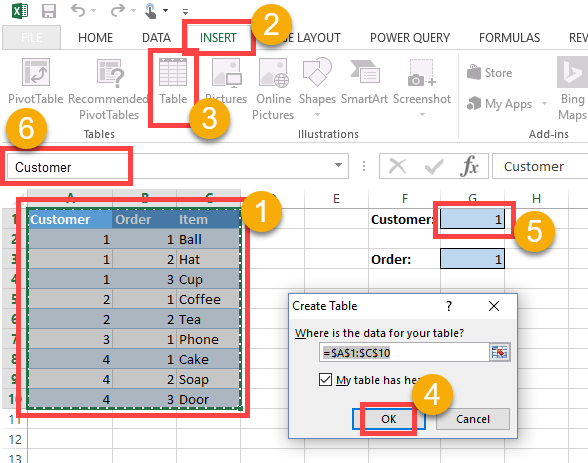
First, we’re going to turn our data into a data table so we can reference it with named ranges. This will allow things to update automatically when we add data to our table.
- Select a cell in data range or highlight the whole range of data.
- Go to the Insert tab in the ribbon.
- Under the Tables section click Table.
- Make sure the range is correct and click OK.
- Now lets also add a named range for our customer input. First select the cell.
- Type in the name Customer into the name box.
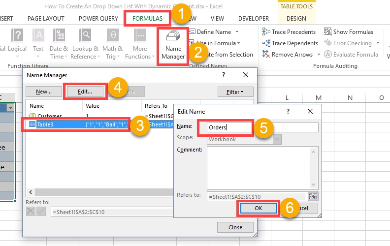
Creating a data table will automatically give the data a named range (something like Table1), so we’ll change the name to something more meaningful next.
- Go to the Formulas tab in the ribbon.
- In the Defined Names section click Name Manager.
- Select the data table you previously created.
- Click on the Edit button.
- Change the name to Orders.
- Press the OK button.
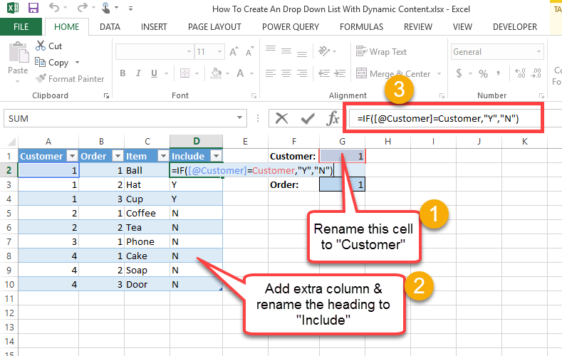
Now we will add an extra column into our data table.
- If you haven’t already done so, change the name to the customer input cell to Customer.
- Add a column to the data table by typing the formula
=IF([@Customer]=Customer,"Y","N")into cell D2. This formula should copy down automatically and a new column heading will be created (something like Column1). Change this heading to something more meaningful like Include by simply typing into the cell. - This formula
=IF([@Customer]=Customer,"Y","N")should appear in each cell in the new column. Check to make sure.
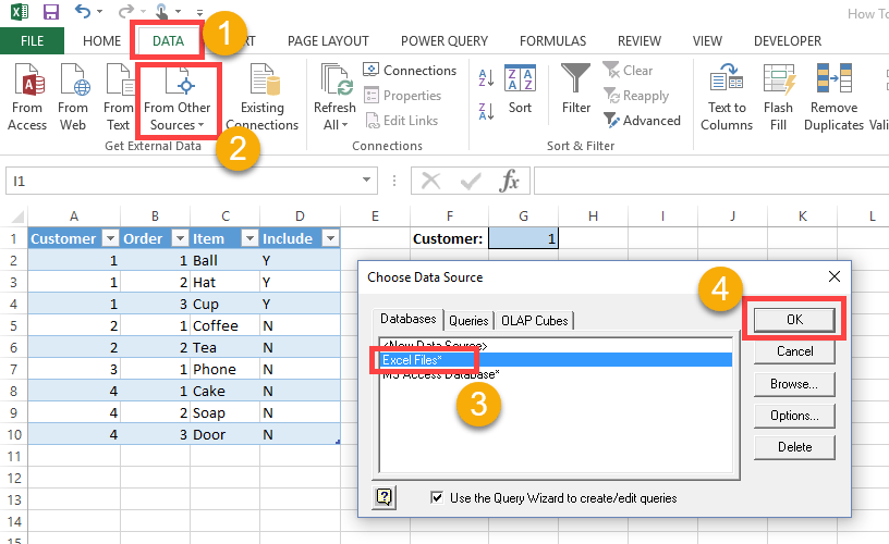
Now we will add a data connection to query our data table and return only the rows of data with Include = Y (i.e. only the rows of data pertaining to a given customer). Before doing this save your workbook.
- Go to the Data tab in the ribbon.
- In the Get External Data section click the From Other Sources button and then choose From Microsoft Query.
- Select Excel Files.
- Hit the OK button.
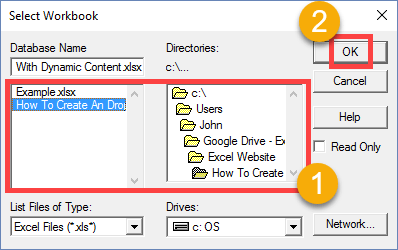
Select this workbook from wherever you saved it and hit the OK button.
Now we will create our query.
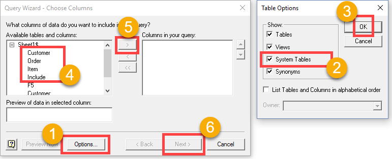
- If you don’t see any available tables and columns, you may need to enable system tables. Hit the Options button.
- Tick the System Tables box.
- Hit the OK button.
- Now you should see you sheet with a list of the column headings in your data table.
- Bring over these columns into the “Columns in your query” section by highlighting them and clicking the right arrow button.
- Click the Next button.
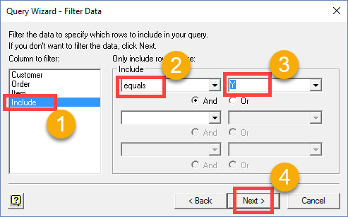
The next screen will allow you to query only the rows pertaining to the customer selected.
- Highlight the Include column in the “Column to filter” section.
- Select equals from the drop down.
- Select Y from the drop down.
- Hit the Next button.
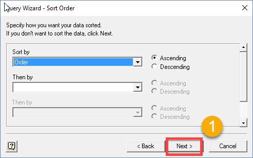
The next screen will allow you to order your query results. For our purposes we don’t need to do this, but it may be helpful to see the orders listed in ascending order in the drop down list we’ll make later so we can add that here. Otherwise, click the Next button.
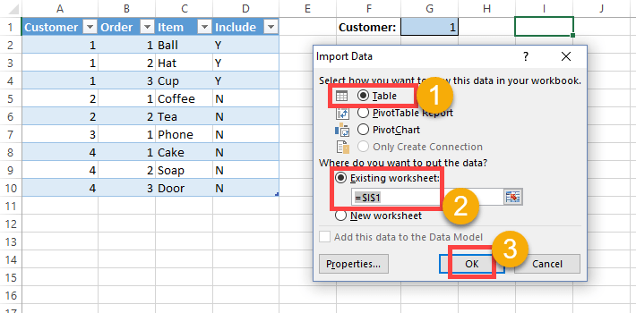
Now choose where your new queried data will appear in your workbook.
- Select Data to appear in a table.
- Select the address in the current sheet. The cell you select will be the upper left most cell of the data, so make sure there is enough room below and to the right of this cell.
- Hit the OK button.
The resulting data will be named something like “Table_Query_from_Excel_Files”, rename this to “Query” using the same method that we renamed our original set of data with.
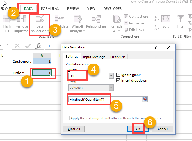
Now let us create the order drop down list.
- Select the cell where you want this drop down list.
- Go to the Data tab in the ribbon.
- In the Data Tools section select Data Validation.
- Select list from the drop down.
- Type
=indirect("Query[Item]")into the field. Note, we had renamed our resulting data from Table_Query_from_Excel_Files to Query - Hit the OK button.
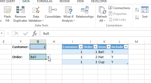
Now when we change the customer and refresh our query, the order drop down list will update with the relevant items.


 👉 Find out more about our Advanced Formulas course!


Nice Tutorial