Power query is amazing data transformation tool! It allows you to import and transform data with ease and helps to create repeatable and robust procedures for your data.
It’s going to save you time and effort if you put in the small amount of time to learn it.
The best part is, it’s built right into Excel 2016 or later. It’s also the same technology that’s used in Power BI, so you’re learning two in demand data skills at the same time!
If you haven’t heard of power query and the awesome things it can do, or you want to fully understand it better, then check out my Complete Guide to Power Query beforehand.
Here are some tips and tricks to help you get the most out of this incredibly useful and easy tool.
Video Tutorial
Delete Steps Until End
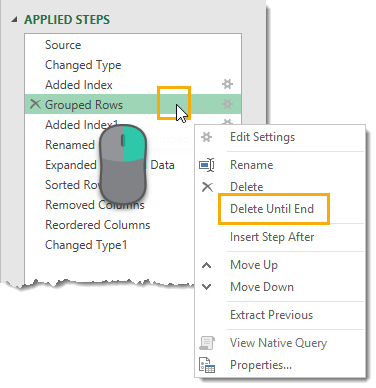
Sometimes when you are building a query with a lot of steps, you end up going down the wrong path. If you’re able to pin point at which step your query started going wrong, then you can delete that step and all steps after to start over (without fully starting over).
In the Applied Steps window pane, right click on the first step you want to delete and then select Delete Until End from the menu.
This will delete that step and all query steps after that step.
Preview or Navigate to Table Objects

A column in your query might contain table objects. If this is the case, the column’s row entries will display the text Table and the data type icon.
You can either preview the table or navigate to it in the query depending on where you click in the cell.

If you click on the blank area of a cell containing a table object, then you will be shown a preview of the table below your query.

When you hover the mouse cursor over the word Table in the cell, it will change to a pointing hand icon. When you click on this part the query, it will add a navigation step to the query which navigates to that particular table.
Double Click to Edit a Query

Editing a query can be done a couple different ways from the Queries & Connections window pane.
- You can right click on the query then choose Edit from the menu.
- You can hover the cursor over the query until the peek window appears, then press the Edit button from the peek window.
The quickest way is to double left click on the query. This will open the query editor on the selected query.
Automatically Add a Row Index to any Query Loaded to a Table

You can add an index column to any query through the power query editor, but it is also possible to add an index row to a query that’s been loaded to a table in a special way. Select a cell in the table output and go to the Data tab and press the Properties button.
Note that the Properties option found in the right click menu of the Queries & Connection pane will open the Query Properties window and not the External Data Properties window that is needed for this tip.

This will open the External Data Properties menu and you can check the Include row numbers option and press the Ok button.
Now the next time you refresh the query loaded to your table, a new column called _RowNum will appear as the left most column and will contain an index for the row number starting at 0.
Change the Default Load Options
When you press the Close & Load button for a query the first time, power query will load the data into an Excel table in the workbook and doesn’t add the data into the data moedel. This is the default load settings in power query.
If you want load the data as a connection only or need to load it into the data model to use with power pivot later on, then you need to select Close & Load To instead and select these options each time you create a new query.
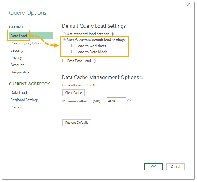
If you find most of the queries you end up creating need to be a connection only or need to load into the data model, then you can change the default load settings. Go to the Data tab then choose Get Data then open the Query Options.
In the Global Data Load settings, choose the Specify custom default load settings option and then select or deselect the desired options.
- Unchecking both the Load to worksheet box and the Load to Data Model box will result in your queries loading as connection only and will not load the data into the data model.
- Checking the Load to worksheet box and unchecking the Load to Data Model box will load queries into an Excel table and not load data to the data model. Note this is the same as when Use standard load settings is selected.
- Unchecking the Load to worksheet box and checking the Load to Data Model box will result in your queries loading as connection only and will load the data into the data model.
- Checking both the Load to worksheet box and the Load to Data Model box will load queries into an Excel table and will load the data into the data model.
Display a Monospaced Font in the Query Editor

It can sometimes be hard to tell if each item in a column of data has the same character length. Not all characters have the same width when using the default query editor font. This can make it hard to tell if you will be able to split a field by character length consistently for the entire column.

Change the font to a monospaced character set by going to the View tab and checking the Monospaced option. This will make it easy to see if things line up in character count.
Navigate Columns with the Arrow Keys

You can select a column by clicking on its column heading. The column will turn to a light green colour when selected and you will then be able to perform various transformations on it by either right clicking on the column heading or using any of the transformation commands from the ribbon.
Once a column is selected, you can navigate to other columns using the left or right arrow keys. In fact, you don’t even need to select a column first, just press the right arrow key and the first column will be selected.
The same trick can be done with rows of data. Once a row is selected from clicking on the row heading you can navigate to other rows using the up or down arrow keys. Again, no need to select a row first, just press the down arrow key and the first row will be selected.
If you select a single cell in a column, you can use the Ctrl + Space keyboard shortcut to select the entire column. You can also use the Ctrl + A keyboard shortcut to select the entire table. Just like in a regular Excel worksheet!
Comments in Power Query Formula Language

You can do a lot with power query just from the UI without ever touching any of the M code that is created behind the scenes. If you do start exploring the M code using the advanced editor (View tab then Advanced Editor), then you’re likely going to want to add comments to your code.
You can do this in two ways.
You can create a single line comment by starting the line with a // double forward slash.
You can create multiple line comments by starting the first line of the comment with a /* forward slash followed by an astrix, then ending the last line of the comment with a */ astrix followed by a forward slash.
Unfortunately, any comments you add into the advanced editor will only be visible in the advanced editor. You won’t be able to see them in the formula bar when navigating through the applied steps of your query.
Add Comments Without Opening the Advanced Editor

It is possible to add comments without opening the advanced editor. Select the step from the applied steps to which you want to add a comment. Add your comment to the end of the step using either comment type and press the Enter button.
The comment will appear visible in the formula bar until you navigate away to a different step or different query. When you come back it won’t be visible in the formula bar any more, but it will still be there in the M code and visible in the advanced editor.
Add Comments that Stay Visible in the Formula Bar

I already said comments are only visible from the advanced editor, but there is a hack to get them to show up in the formula bar.
Write your comment inside a formula instead of at the end of the step. You’ll need to use the opening /* and closing */ comment characters as the comment will need to be closed so the rest of the formula is not considered as part of the comment.
This will remain visible in the formula bar when navigating through the applied steps of your query.
Add Comments with the Query Step Properties
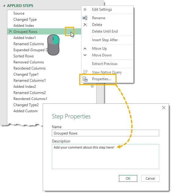
You can add comments to any of the query steps listed in the applied steps window pane using the query’s properties window. Right click on the query and select Properties from the menu.
You’ll be able to add a description to the step. This description will appear as a single line comment above the M code for the step in the advanced editor.
You can also change the name of the step from this window. This will change the references for the step in the advanced editor as well.
Create a Sequential List

Creating a sequential list object in power query is easy when you know how. Add a custom column with the following formula for a list starting at 5 and ending at 10.
={5..10}
This will even work by referencing columns instead of static hardcoded numbers. Use a formula similar to the following where [Start] and [End] are two whole number columns in your query.
={[Start]..[End]}
If either the Start or End column is a decimal number, the expression will result in a error.
If the Start number is greater than the End number, the expression will result in an empty list.
Avoid Case Sensitivity with Filters
Power query is case sensitive. This can cause errors in your data analysis down the road if you’re not careful.
If you filter out the item Keyboard from your data and later it shows up as keyboard in the source data, then your query won’t filter out the lower case version.

This can be avoided by transforming a column to upper case before applying any filters.
We can also retain the original case in our data by using the UPPERCASE transformation found in the Add Column tab. This will create a new column with the upper case values while keeping the original column intact.

Now we can apply any filter on the uppercase version of the column and then delete the column after. This allows us to apply a case insensitive filter without altering the case in our data.
Double Click to Rename a Column

You’re probably going to be renaming a lot of columns during your power query career so you’re going to want to learn the quickest way to do it. A double left click on the column heading will allow you to quickly change a column’s name.
Rename a Column with a Keyboard Shortcut
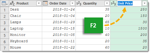
You can rename a column using a keyboard shortcut. This one is a bit slower, but worth knowing for those that prefer the keyboard to the mouse. With the column selected, press F2 on the keyboard and you can rename the column heading.
Navigate Through Complex Query Dependencies
This feature can be a life saver when your workbook starts to get overloaded with queries. It can be easy to forget what query is using what data source and which queries depend on each other.

Go to the View tab and press the Query Dependencies command to open the query dependencies viewer. This will give you a visual representation of all the queries in the workbook along with their precedents and dependents.

There’s a lot going on in the Query Dependencies window.
- You’ll be able to see your data sources. These are the smaller boxes in the window and will have a larger icon indicating the type of source data.
- Left click on any item and it will turn a light green along with all its dependents and precedents.
- Right click on any item and a menu will appear with the option to center the view on that item or center the view on all the precedent and dependent items.
- Left click and drag any empty area to move the view around.
- You can change the layout to show dependencies from top to bottom, bottom to top, left to right or right to left.
- You can zoom in or out on the view manually using the zoom bar. Another way you can zoom in on the view is using the mouse scroll wheel if yours is equipped with one. Another option is to double left click on any empty area to zoom in.
- You can fully zoom out on the view using the zoom out button on the lower right.
Drill Down to a Single Value
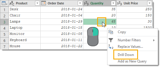
Drill down to any single item in your query. Right click on the cell and choose Drill Down.
Depending on your data, this could be a single value, list or a table. This can be useful for creating a single value from your data which you can reference in a custom column calculation.
Enable Fast Data Load in Power Query
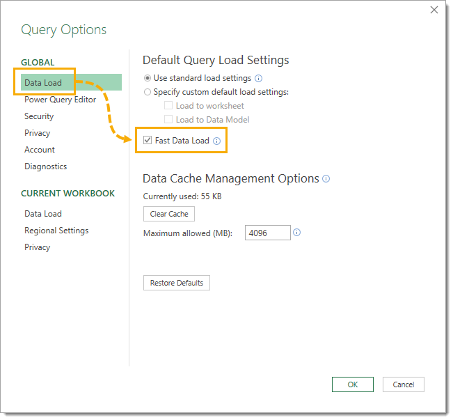
Faster is always better, right? If your queries are slow, you can enable the fast data load option to speed them up. Go to the Data tab and press the Get Data button, then open the Query Options.
Go to the Global Data Load settings and check the Fast Data Load box. Your queries will take less time to load, but Excel may become unresponsive during the loading.
Disable the Auto Detect Data Type Feature

When you import data into Excel with power query, Excel will guess what data type each column is based on the first few hundred rows. Power query will then automatically create query steps to promote the first row to column headings (for CSV files) and change data types.
If you prefer to control the data type selection and not have excel automatically create this steps for you, then you can disable this option.

To open the query options, go to the Data tab then Get Data then choose the Query Options.
Go to the Current Workbook Data Load settings and check the box to Automatically detect column types and headers for unstructured sources.
Next time you create a query, you won’t see any steps other than the source step.
Explore Power Query’s Function Library
Power query’s M code language is a functional language. This means the M code is mostly built with functions that do specific things based on their inputs. Writing M code in power query is like building with Lego, there are many different types of Lego pieces and each piece is designed for a specific purpose.
M code comes with a large selections of functions to use. In fact you can explore the entire library of available functions from within the power query editor.
![]()
Create a new blank query, go to the Data tab and press the Get Data command then choose From Other Sources then choose Blank Query. Now in the formula bar enter =#shared and press Enter.

Power query will then show all the items available to the workbook. This will include all the power query functions!

If you click on any of the functions listed, you’ll be taken to a mini help guide for that function.
- The function name is shown.
- There is a brief description of what the function does.
- You can test out the function on your data.
- The functions syntax is shown.
- There is a simple example shown to demonstrate the input and output of the function.
Split a Query into Two Parts

Maybe your query is getting too long, or maybe you want to use the first part of it as a source in other queries. If this is the case, you can split up a query into two parts.
Right click on the step on which you want to divide the query then choose Extract Previous from the menu. This will extract the steps before the selected step into a new query. You’ll then be prompted to name the new query.
The remaining steps will then reference the new query as its source.
Copy and Paste Queries to a New Workbook

If you need to reuse a power query from a previous workbook, you can easily copy and paste it from the old workbook to the new workbook.
In the Queries & Connections window of the old workbook, select the queries you want to copy then right click and choose Copy from the menu. Now navigate to the new workbook and right click in the Queries & Connections window and choose Paste from the menu.
This will copy all the selected queries along with all the queries they reference.
If any of the copied queries, or the queries they depend on, reference a table in the old workbook then those queries will show a Download did not complete error message. You will need to copy over those tables into the new workbook separately to fix this.
Double Click to Rename a Query

You can quickly rename any query from the query list pane on the left hand side of the query editor. Double left click on the query which you want to rename, then type in the new name and press Enter to confirm the change.
Double Click to Hide or Show the Query Editor Ribbon

If you find the ribbon in the power query editor is getting in the way, you can hide. Double left click on any of the ribbon tabs to hide the ribbon. Double left click on the tab again to show the ribbon.
Yep, this is the same trick from the regular workbook ribbon but it can also be used in the power query editor!
Disable Relationship Detection

This is another tip that can potentially speed up your power query queries.
When you load data into the data model from power query, Excel will try to find and build relationships between the new data and other tables in the data model. This extra processing step will slow down your queries.
If you are always loading your data into the data model then you might want to turn this feature off to save time. Go to the Data tab then press the Get Data button and open the Query Options.
In the Current Workbook Data Load settings, uncheck the Create relationships between tables when adding to the Data Model for the first time option. This will prevent Excel from creating the relationships between tables in the data model.


Thanks for the article .. that was helpful …
Looks great!
Extremely well put together – a great help for those exploring the possibilities of Power Query! Thank you.
No problem Roland!
+1 @Roland
w.r.t. comments in Advanced Editor: if a comment line is immediately above a step it will turn into a tooltip when you hover over the step name in the “Applied Steps” pane.
Also the query code itself is UNICODE so you can use symbols in step names. Usually this is overkill, but you can use it to draw attention to things like debugging steps.
Great tips Steve, thanks!
Hi John, Thanks for tips. How does one change a query that has already been loaded but realise there afterwards that it only needs to be a connection? I can only think of duplicate / edit – then change the connection and delete the original. Have yet to try that as I have many to do (to reduce the extra sheets not needed…)
Just delete the table it loaded to from the workbook. The query will become a connection only.
You can also change things by right clicking on the query in the query and connections window pane and selecting load to from the menu.
Thank You
Very Good
Great tips, thanks.
No problem Martin!
Great material!, thanks a lot
Hi John, I am loading a power query to a table and then adding additional columns to the table to perform calculations. When I refresh the query, it takes a significant time because it is calculating during the background refresh. I turned off Automatic Calculations but it continues to calculate. I would like it to refresh the table from the power query and then calculate the columns I have added. Any ideas? Thanks
The only thing I can think of is to delete all the formulas, except for those in the first row before refreshing. Then copy down the formulas from the first row after refresh.
Are you aware of a way (or any third party editor or plugin) that allows you to open the Power Query Advanced Editor for a given Excel file without all the clicks? We have found Power Query really useful, but cumbersome to work with given that it takes about 5 clicks to get to the Advanced Editor, which is generally where we want to be.
Sorry, not aware of anything. You can copy queries from the queries and connection pane into a text editor and this will give you the M code.
Thanks – it feels like something Microsoft needs to solve if they want better adoption of this technology. Would be great if you could open an Excel file with Visual Studio and edit the embedded M code in an editor that has syntax highlighting, Intellisense, etc. It’s surprising to me that nothing like that exists.
I did find one useful shortcut that is worth sharing. You can reduce the number of clicks to get to the editor if you add the “Launch Power Query Editor” command it to the Quick Access Toolbar. Helps alleviate some pain at least…
Hello-we are using one of these at work but the folks using it are asking if there is a way to add a column that they can put notes in for each row that will stay with that row as it refreshes. For us, each row is a work order and it would help immensely with work planning. If it cant-are you aware of any other way to pull and refresh data from a source that does allow for a comment column?