Do you want to know how to display your negative numbers as red font color in Microsoft Excel?

It’s actually quite easy!

The formatting features in Excel are quite powerful, and they allow you to conveniently spot and highlight important facts about your data such as negative numbers.

Losses are usually displayed as red numbers in financial reports such as a company profit and loss statement. This red font color helps to make them easier to see.

But you can also use these same techniques to show your negative values in any color of your choice.

This post is going to show you all the different ways you can use to display your negative numbers with red font color in Microsoft Excel.

• Show negative numbers as red using a number format.
• Show negative numbers as red using a custom number format.
• Show negative numbers as red using conditional formatting.
• Show negative numbers as red using VBA.
• Show negative numbers as red using Office Scripts.

Download your copy of the example workbook with the above link and follow along!

Display Negative Numbers as Red with a Number or Currency Format

The most straightforward method to show your negative numbers in red font color is to use a number or currency format.

Both the number and currency formats have options to show negatives with red font color.

Follow these steps to apply the number or currency format to your numbers.

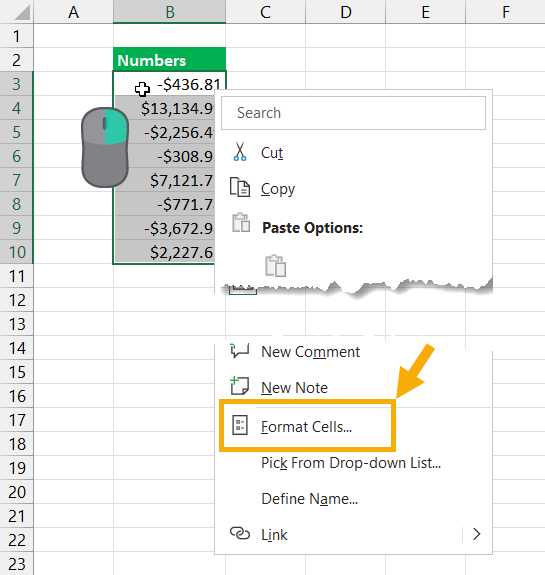
1. Select the cells to which you want to apply the custom format.
2. Right click on the selected cells and choose Format Cells.

You can also use the Ctrl + 1 keyboard shortcut to open the Format Cells dialog box.

3. Select the Number tab inside the Format Cells dialog box.
4. Select Number or Currency from the Category options.
5. Select the example with red font in the Negative numbers section.
6. Press the OK button.

Any cells you apply this format to will automatically change to a red font color whenever the value is negative.

This is great when your values are derived from a formula and might change often as you don’t need to manually update the color.

Display Negative Numbers as Red with a Custom Format

Excel also allows you to define your own custom format from the Format Cells dialog box.

You’ll be able to define number formats and colors for positive, negative, and zero values. This includes the ability to specify a font color for the displayed format, so your positive values can be green while your negative values are red.

Follow these steps to create a custom format.

1. Select the cells to which you want to apply a custom format.
2. Open the Format Cells menu. Right click and select Format Cells from the options, or press the Ctrl + 1 keyboard shortcut.

3. Go to the Numbers tab.
4. Select Custom from the Category section.

[Green]$#,##0.00;[Red]-$#,##0.00;$0.00

5. Add the above format code to the Type input.
6. Press the OK button.

After you press the Ok button, your custom format will be applied and you will see the various format options applied to your positive, negative, and zero values.

The format string entered is made up of several parts.

1. The formats for positive, negative, and zero values are separated by a semi-colon; character.
2. The format string for positive values is first. You can specify a color [Green] inside square brackets before the number format string.
3. The format string for negative values is second. You can specify a color [Red] inside square brackets before the number format string.
4. The format string for zero values is third. You can also specify a color, but the example used in this post doesn’t specify any color and will use the default font color so any zero values will display in black.

One great thing worth mentioning about the custom format option is there are several preset options available that include a red negative color. This way you can avoid writing the syntax from scratch, and can instead customize one of the existing options.

Display Negative Numbers as Red with Conditional Formatting

Conditional formatting is a feature that allows you to set the format of a cell, based on customizable rules.

With conditional formatting, it’s possible to change any type of cell formats such as borders, font size, font style, fill color, and much more.

You can also use this to change the font color to red when the cell value is less than zero.

Follow these steps to apply conditional formatting to your range of numbers.

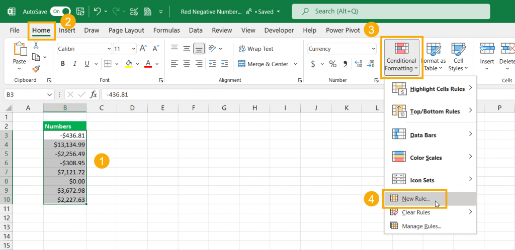
1. Select the range of cells to which you want to apply conditional formatting.
2. Go to the Home tab.
3. Select the Conditional Formatting command from the Styles section.
4. Choose New Rule from the menu options.

This will open up the New Formatting Rule menu where you can select from various different types of rules to create.

5. Choose the Format only cells that contain option under the Select a Rule Type section.
6. Choose Cell Value and less than in the dropdown options, then add 0 into the input box on the right.
7. Press the Format button to choose what formats will be applied when the rule is true.

This will open up a simplified version of the Format Cells dialog box which only contains the Number, Font, Border, and Fill tabs.

8. Go to the Font tab.
9. Select a Red from the Color dropdown menu.
10. Press the OK button.

This will open up the New Formatting Rule menu again, but this time the Preview window will show a preview of the selected formats that will be applied when your rule is true.

11. Press the OK button to save your new conditional formatting rule.

You will now see any values that are less than zero in your selected range appear with red font color.

There is one interesting advantage about using a conditional format rule to display your negatives in red. You can apply different number formats such as percentage to your numbers through the regular formatting options, and then control the font color with a single rule.

With conditional formatting, you also get more color options than with a custom format.

There are many preset color options available to choose and you can even choose a color based on RGB or Hex code for the ultimate color customization possibilities.

Display Negative Numbers as Red with VBA

All the previous methods discussed are dynamic, if the numbers change so will the format to reflect the new value.

But perhaps you want a static solution but without manually changing the font color for each cell.

This is where you can use a VBA solution to automate the process.

VBA is the scripting language baked into Excel, and it’s able to automate many tedious tasks.

Press Alt + F11 on your keyboard to open the VBA code editor.

Then you can go to the Insert menu and select Module from the options. This will create a new module where you can add your VBA code.

Sub ChangeFontColor()
Dim rng As Range

For Each rng In Selection
    If rng.Value < 0 Then
        rng.Font.Color = vbRed
    Else
        rng.Font.Color = vbBlack
    End If
Next rng
End Sub

Copy and paste the above code into the new module.

This code will loop through the selected range in the workbook and test if the value in the cell is less than zero.

When the value is less than zero, it will apply a red font format to the cell. Otherwise, it will apply a black font format.

Now you can run this code at any time to apply red font color to the numbers in your workbook.

1. Select the range of cells to which you want to apply red font color to any negative values.
2. Press Alt + F8 on your keyboard to open up Macro dialog box. This will show you all the VBA scripts in your workbook and you will be able to run any of them.
3. Select the ChangeFontColor from the list of available macros.
4. Press the Run button.

The code will execute and change any font colors according to the values of the cells.

The font color results will be static, so if the numbers change you will need to rerun the VBA script to update the font colors.

Display Negative Numbers as Red with Office Scripts

There is also another option for an automated static solution.

Excel has a new modern scripting language based on the TypeScript language. This is a superset of the JavaScript language which runs the web.

The new Office Script language is available in Microsoft 365 business plans and can be run from the online web version of Excel.

Open Excel Online and go to the Automate tab, then click on the New Script button to open the Office Script editor.

This will open the script editor on the right side of the Excel window with a blank script.

You can click on the generic name given to the script and rename with descriptive name so you can easily find and run it later.

function main(workbook: ExcelScript.Workbook) {

  //Create a range object from selected range
  let selectedRange = workbook.getSelectedRange();
  //Create an array with the values in the selected range
  let selectedValues = selectedRange.getValues();
  //Get dimensions of selected range
  let rowHeight = selectedRange.getRowCount();
  let colWidth = selectedRange.getColumnCount();

  //Loop through each item in the selected range
  for (let i = 0; i < rowHeight; i++) {
    for (let j = 0; j < colWidth; j++) {
      if (selectedValues[i][j] < 0 ) {
        //Change font to red color when value is less than zero
        selectedRange.getCell(i, j).getFormat().getFont().setColor("#FF0000");
      } else {
        //Change font to black if value not less than zero
        selectedRange.getCell(i, j).getFormat().getFont().setColor("#000000");
      }
    }
  }
};

You can then paste the above code into the Office Script editor and then click the Cloud icon to save it. There is also a Run button that will allow you to run the script.

This script will loop through the selected range in the workbook and test if each value is less than 0. If the value is negative, it will change the cell font color to red. Otherwise, it will change the cell font color to black.

You can run the script by going to the Automate tab and selecting the All Scripts command to open up a list of the scripts you have created.

Click on the desired script.

This will open up a window focused on the script containing a Run button.

Select the range of numbers to run the script on then press the Run button and the negative numbers will get a red font color applied.

Conclusions

There are many ways to implement red negative numbers in Microsoft Excel.

Easy options such as the number and currency formats are easy to implement but have no other color choices available other than red.

Custom formats will allow you to choose different colors and number formats for positive, negative, and zero values but the available color choices are limited.

If you want to choose a specific shade of red or any other custom color, using conditional formatting will be your best bet as any color can be obtained using RGB or Hex codes.

These format options are all dynamic and the formats will update accordingly if the values in the cells change. If you need a static solution, you can avoid the manual cell formatting by using either a VBA or Office Scripts to automate the process.

Have you ever needed to display your negative values in red? Which method do you prefer? Let me know in the comments below!