If you’re working with large sets of data in Excel, then it’s a good idea to add a serial number, row number or ID column to the data.

A serial number is a unique identifier for a row or record of data and they will usually start at 1 and increase incrementally with each row.

This way you can refer to each record in your data set by the serial number.

In this post, I’ll show you 15 interesting ways which you can add row numbers to your data.

Use the Row Headings

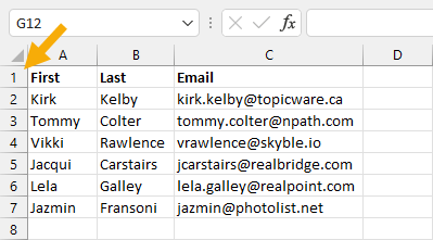
Good news! Excel comes with serial numbers out of the box.

On the very left hand side of every sheet is the row heading with row numbers in an incrementally increasing sequence.

You can use these as serial numbers for your data.

Pros

• You don’t need to do anything to create them as they are there by default.
• These numbers will adjust when you delete or insert a row.
• Works inside Excel Tables.

Cons

• You can’t change them.
• You need to position your data starting in cell A1.
• If your data contains column headings, then the row number will start at row 2 for the first record.

Use the Fill Handle

This one is an amazing trick!

Once you learn it, there is no going back to the old way of manually typing each number of a sequence.

The fill handle will automatically create a sequence of serial numbers for you with just a click and drag.

You first need to enter two sequential numbers.

Notice the active cell has a square in the lower right?

This is the Fill Handle and you can use it to automatically fill in the rest of the sequence which you started to add manually.

Select the first two cells and then hover your mouse cursor over the lower right corner until it turns into a small black plus sign. Then click and drag down to the end of your data.

If you’re working with a large data set, then click and drag might not be feasible. In this situation, you can double click on the fill handle to fill the sequence down to the end.

When you release the fill handle this will fill in the sequence of numbers and a small fill handle options menu will appear at the bottom right of your filled sequence.

There is one handy option in this menu that allows you to avoid filling down any cell formatting.

Click on the menu options and choose Fill Without Formatting and any copied cell formatting will be removed.

Pros

• Easy to use and only requires manually entering two values.
• The serial number entered in a row will not change once it’s entered.
• Deleting or inserting a row won’t affect other record ID’s.
• Works inside Excel Tables.

Cons

• Each time you add new rows to the bottom of your data table you will need to manually add a serial number or repeat the fill handle process.
• For large data sets, clicking and dragging the fill handle to the end can be tedious.

Use the Fill Series Command

This option is very similar to the fill handle method, but doesn’t require and long click and drag actions down the length of your data.

Add the first two serial numbers to your data set. Then select the entire range of cells which you would like to fill including the two serial numbers you have already entered.

To select a longer range, it’s easier to start at the bottom and select up to the top.

If you place the active cell cursor in the next column which contains data, you can use Ctrl + Down to get to the last cell. Move the cursor back over to the ID column, then Use Ctrl + Shift + Up to select all the blank ID cells. Then use Shift + Up to select any previously entered serial number cells.

Go to the Home tab of the ribbon and click on the Fill command then choose Series.

This will open the Series menu.

1. Choose Columns for the Series in option.
2. Choose AutoFill for the Type option.
3. Press the OK button.

This will fill in the remaining series in your selected blank cells.

Pros

• Easy to use and only requires entering the first two numbers manually.
• No long click and drag actions required.
• You can delete or insert rows without affecting other existing serial numbers.
• Works inside Excel Tables.

Cons

• This is not a dynamic solution, so when you add new rows to your data table you will need to manually add a serial number or repeat the fill process.

Add One to the Previous Number

This is the intuitive method to adding a series of numbers to your data. Excel’s is designed to calculate, so adding 1 to the previous serial number is no problem.

= B3 + 1

Enter the value 1 into the first row of your data. Then in the next row enter the above formula. In this example B3 is the cell directly above.

Now you can copy and paste this formula down the remaining rows. To do this quickly, double click on the fill handle of the cell which contains the formula.

Pros

• Easy to implement.
• Easy for someone to understand what the formula is doing.
• You can copy and paste the formula down when new rows are added.

Cons

• If you delete any row, you will get #REF! errors for all rows below as you are deleting a cell that is referenced by those cells below.
• The formula is not consistent for the entire column since the first row needs to contain a hard coded value of 1.

Use a Relative Reference Named Range

This method is going to use the same idea where you add 1 to the previous serial number, but it is going use a clever trick to make it more robust.

What you need to do is create a named range that will always refer to the cell above it.

Then you can reference this named range instead of a direct cell address like B3.

Go to the Formulas tab and click on Define Name.

This will open the New Name menu. Give your named range a name like Above, this is how you will reference it inside formulas later.

= INDIRECT ( "R[-1]C", FALSE )

Add the above formula in the Refers to section of the New Name menu then press the OK button.

This formula uses the INDIRECT function with row and column notation. R[-1] indicates the reference is one row above the current cell.

Now when you use the Above name inside a formula it will reference the cell directly above the cell which you are entering the formula.

= SUM ( Above, 1 )

Enter the above formula into the first row and then copy and paste it to the end of your data.

Using the SUM function is a small improvement to the previous method as there is no need to enter a value in the first row. The formula can be applied consistently for each row.

The SUM function will count text values as zero, so you can safely reference the column headings when the formula is in the first row without producing a #VALUE! error.

Pros

• You can copy and paste the formula down when new rows are added.
• Use the same formula for the entire row.
• Works well inside Excel tables.
• Serial numbers will dynamically adjust when you delete or insert a row.

Cons

• Takes more time to set up.
• The formula might not be as obvious to someone else looking at your spreadsheet,
• The named range uses the INDIRECT function which is a volatile Excel function. They can slow down your Excel workbook because they are recalculated more frequently.

Use the ROW Function

There is an Excel function that can return the current row number and it’s perfect for creating serial numbers.

= ROW ( ) - ROW ( $B$2 )

Add the above formula, where B2 refers to the column heading cell, into the first row and copy and paste it down.

The ROW function returns the row number of the current row when no argument is passed to it. In order to start the serial numbers at 1, we then need to subtract off the row number of the column heading cell. This is accomplished using an absolute reference to the cell with the column heading.

Pros

• Easy to implement.
• Inserting or deleting a row won’t cause any errors and serial numbers will update accordingly.
• Works inside Excel Tables.

Cons

• The formula needs to reference the column heading cell with an absolute reference.

Use the COUNTA Function

This is another formula option that will rely on counting previous rows of data.

In order to use this formula, you will need a column that will never contain blank values as the COUNTA function does not count empty cells.

= COUNTA ( $C$3:C3 )

Enter the above formula into the first row and then copy and paste it to the end of your data. In this formula C3 is a cell in the first row but another column which will not contain any blank values.

Notice the range reference in the formula contains a partial absolute reference with the $ symbol. This causes the formula to include all records above the current record in its count as it gets copied down the data set.

Pros

• Easy to implement where the only tricky part is adding the partial absolute reference.
• You can insert or delete rows without errors.
• Works with Excel Tables.

Cons

• You need to refer to another column which can’t have any blank values.

Use the SUBTOTAL Function

The SUBTOTAL function is interesting because it can return values based on what cells are visible.

It can also be used to perform other aggregations like a count and not just a sum.

This means you can use it to create serial numbers that change based on filtered data.

= SUBTOTAL ( 3, $C$3:C3 )

Add the above formula into the first row then copy and paste it down the data.

This formula works exactly like the COUNTA method, because it is the same. The first argument in the SUBTOTAL function tells Excel to use a count type aggregation.

The only difference is when you filter your data, the serial numbers will update based on what is still visible.

Pros

• Same pros as COUNTA method.
• You can use filters on your data and they will dynamically change the serial numbers.

Cons

• Same cons as COUNTA method.
• The SUBTOTAL function is less known by most Excel users.

Use the SEQUENCE Function

The SEQUENCE function is a new dynamic array function. This means one formula can produce an array of values.

It can do a lot more, but this function can also generate a single column of increasing numbers that start at 1. Perfect for serial numbers!

= SEQUENCE ( COUNTA ( C3:C8 ) )

Add the above formula into the first row of data. In this example C3:C8 is the entire range of a column. This will determine how many serial numbers the SEQUENCE function will return.

= SEQUENCE ( 6 )

Another approach is to hard code the row count inside your SEQUENCE function like the above formula. Unfortunately, this method would mean you need to manually adjust the count each time you add or remove rows of data.

Pros

• You only need one formula. No need to copy and paste a formula down to the end of your data set.
• Inserting or deleting any row other than the first one won’t produce any errors and your serial numbers will adjust accordingly.

Cons

• Deleting the first row will delete all the serial numbers.
• Can’t be used inside Excel Tables.
• If you add rows at the bottom of your data set, you will need to adjust the range reference in the SEQUENCE function to include these.
• The COUNTA function will require non blank values.

Use Power Pivot

This one is a bit weird since it will create serial numbers inside a pivot table.

But it may be just what you’re lookin for.

You can use power pivot with a calculated column to number your pivot table rows.

Select your table of data and go to the Power Pivot tab and click on Add to Data Model.

= RANK.EQ( Data[Email], Data[Email], ASC )

This will open the power pivot add-in and you’ll be able to add the above formula into the table.

In this example, the table has been named Data and we are ranking the Email column which contains unique text values. This results in column that can be used as a serial number.

To use this calculated column inside a pivot table.

1. Go to the Insert tab.
2. Click on PivotTable.
3. Choose From Data Model from the options.
4. Choose the location you would like to place the pivot table.
5. Add add the fields into the Rows area of your new pivot table including the Rank calculated column.
6. Go to the Design tab ➜ Report Layout ➜ Show in Tabular Form. This will make it look more like a dataset instead of a pivot table.

Pros

• You can create serial numbers inside a pivot table.

Cons

• You need a column with unique values like an email.
• Results are not ordered.

Use VBA Code

VBA has been in Excel and other Office applications for a long time.

It was the go to method for automating any task in Excel. So you can certainly use it to automatically generate your serial numbers.

These days, there are usually much better options available and I would only recommend using a VBA solution as a last resort.

Sub AddSerial()

Dim cell As Object
Dim count As Integer
count = 0

For Each cell In Selection
    count = count + 1
    cell.Value = count
Next cell

End Sub

Add the above code into the visual basic editor.

1. Pres Alt + F11 to open up the visual basic editor.
2. Right click inside the VBAProject window.
3. Select Insert from the menu.
4. Select Module from the submenu.
5. Paste the code into the module.

The above code will add an increasing sequence of numbers starting at 1 into any selected range.

Now you can run the code.

1. Select the entire column which you want to add serial number into.
2. Press Alt + F8 to open the Macro dialog box.
3. Select the macro to run.
4. Press the Run button.

This will fill your selected range with a sequence of numbers starting at 1.

Pros

• Adds static numbers into any range.

Cons

• Uses VBA and will require the workbook to be saved as an xlsm file.
• Hard to set up and run.
• You will need to re-run the code if you add or insert rows to your data set.

Use an Index Column in Power Query

Power Query is an amazing data transformation tool found in Excel and other Microsoft products.

If you’re already using it to import your data from an external source into Excel, then it might be the perfect solution to adding serial number to your data.

If your data is already in Excel, you can still use power query to add serial numbers but you will need to add your data into an Excel table first.

I wrote a detailed article about Excel Tables, where you can learn all about them including how to convert your data into a table.

Add your data into query by using a From Sheet query. Select a cell inside your table ➜ go to the Data tab ➜ choose From Sheet.

This will open up the power query editor and you will be able to add a column with serial numbers from here.

Go to the Add Column tab and click on the Index Column command. Click on the small arrow icon of the Index Column button to choose to start the index From 1.

Now you can go to the Home tab ➜ Close & Load ➜ Close & Load To ➜ Choose to load the results into an Excel table and pick the location to load it to.

Your data will be loaded into another table with an extra index column.

If you add or remove data from the source, you will need to refresh the query output to see the updated results. You can refresh the query by right clicking on the table and choosing Refresh from the menu options.

Pros

• Great option if you’re using power query to import your data from an external source already.
• Easy to refresh once it is set up.

Cons

• Power query can be intimidating to someone using it for the first time.
• It doesn’t add the serial numbers into the data source, it will only add them to the output of a query on the data source.

Use the Connection Properties for Connected Tables

If your data has been loaded into a table from an external source like power query or an exported SharePoint list, then you can enable row numbers from the connection properties menu.

Select your connected table and go to the Data tab and click on the Properties command.

This will open the External Data Properties menu and you can enable the option to Include row numbers and press the OK button.

Now you need to refresh the connection in order to see the row numbers. Go to the Data tab and click on the Refresh button.

After refreshing the connection, you will see a new column in the table called _RowNum which starts the count at 0.

Pros

• You can delete or insert rows in the source data and the row number will update when you refresh the connection.

Cons

• This feature only works with connected data tables.
• The row numbers setting is hard to discover.
• The row number column can only appear as the very left column in the table.
• The row numbers start at 0 and can’t be changed to start at 1 instead.
• The column heading for your serial numbers can’t be changed from _RowNum.

Use Office Scripts

Office Scripts is a new TypeScript based scripting language which is currently only available in Excel online for Enterprise Microsoft 365 plans.

This is the replacement for VBA and you can certainly use it to auto generate a set of row numbers.

You will need a few things in order to use this method first.

• Your Excel file has to be saved in SharePoint.
• You need to open your Excel file in the Excel web application.
• You need to be on an enterprise level Microsoft 365 plan.
• The Office Scripts feature needs to be enabled by your IT admin.

Open your file in Excel online then go to the Automate tab and click on New Script.

function main(workbook: ExcelScript.Workbook) {
	let selectedSheet = workbook.getActiveWorksheet();
	let myID = selectedSheet.getRange("Data[ID]");
	let myCellCount = myID.getCellCount();
	let mySerialNumbers = new Array(Array(myCellCount));
	for (var i = 0; i < myCellCount; i++) {
		mySerialNumbers[i] = [i+1]
	}
	selectedSheet.getRange("Data[ID]").setValues(mySerialNumbers);
}

Paste in the above code into the Code Editor. You can rename the script and press Save Script to save the script.

Press the Run button in the Code Editor to run the script.

This script relies on your data being inside an Excel Table named Data with a column named ID.

Pros

• Once this is set up, its very easy to use.

Cons

• Excel file needs to be saved in SharePoint.
• Office Scripts are only available in Excel online for Enterprise Microsoft 365 plans.
• You can only run this script from Excel online.

Use Power Automate

Now that you have an Office Script to add serial numbers to Excel, you can use Power Automate to automate the running of this script.

You can use power automate to run this script on a schedule, so you can automatically update your serial numbers every day or even every hour.

1. Log into https://flow.microsoft.com/
2. Click on Create in the left hand navigation pane.
3. Click on Scheduled cloud flow.
4. Give your flow a name like Add Serial Numbers.
5. Set the start date to today’s date and time.
6. Set the frequency which you would like the flow to run.
7. Click on the Create button.

Now add a Run script step to the flow and select the file and script to run then Save the flow.

This will now automatically run the script to add serial number at your desired frequency.

Pros

• The solution automatically runs in the background.
• You can work on the file in the desktop or web app while the flow runs.

Cons

• Requires a complex setup.
• Needs Microsoft 365, SharePoint and Office Scripts.

Conclusion

There are a ton of options when it comes to adding serial numbers to your data in Excel.

Each method will have various pros and cons that might make them a better option for your use case. It’s worth exploring them all to see which will work best for you.

Whatever your skill set there is an option for you that will get you your desired results.

Did I miss your favourite way to add row numbers in this post? Let me know in the comments if you have another method you use!