How To Generate A List Of Sheet Names From A Workbook Without VBA

Posted by John | Dec 7, 2016 | Tips & Tricks | 41 |

In this post we’ll find out how to get a list of all the sheet names in the current workbook without using VBA. This can be pretty handy if you have a large workbook with hundreds of sheets and you want to create a table of contents. This method uses the little known and often forgotten Excel 4 macro functions. These functions aren’t like Excel’s other functions such as SUM, VLOOKUP, INDEX etc. These functions won’t work in a regular sheet, they only work in named functions and macro sheets. For this trick we’re going to use one of these in a named function.

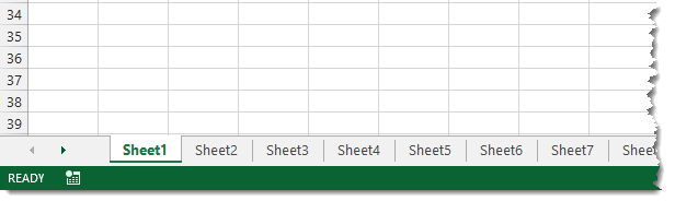
In this example I’ve created a workbook with a lot of sheets. There are 50 sheets in this example so I was lazy and didn’t rename them from the default names.

Now we will create our named function.

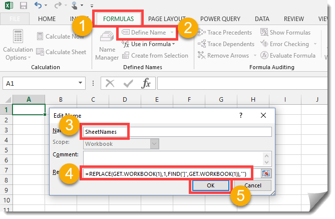
Go to the Formulas tab.
Press the Define Name button.
Enter SheetNames into the name field.

Enter the following formula into the Refers to field.

=REPLACE(GET.WORKBOOK(1),1,FIND("]",GET.WORKBOOK(1)),"")

Hit the OK button.

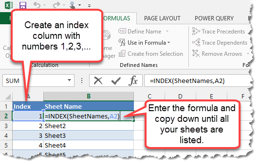
In a sheet within the workbook enter the numbers 1,2,3,etc… into column A starting at row 2 and then in cell B2 enter the following formula and copy and paste it down the column until you have a list of all your sheet names.

=INDEX(SheetNames,A2)

As a bonus, we can also create a hyperlink so that if you click on the link it will take you to that sheet. This can be handy for navigating through a spreadsheet with lots of sheets. To do this add this formula into the column C.

=HYPERLINK("#'"&B2&"'!A1","Go To Sheet")

Note, to use this method you will need to save the file as a macro enabled workbook (.xls, .xlsm or .xlsb). Not too difficult and no VBA needed.

41 Comments

Kinsen on 2017-12-22 at 15:01

Hi,
this is very helpful, but it would be great if you mention how to do this only for visible sheets?
Reply
- John on 2017-12-23 at 14:13
  
  Unfortunately, with this method it’s not possible.
  Reply
andrew on 2018-01-10 at 10:51

The hyperlink doesn’t work when there are spaces in the worksheet names
Reply
- Rajid ALi on 2018-01-17 at 00:49
  
  Exactly…. any solutions ????
  Reply
- John on 2018-01-17 at 09:44
  
  When there is a space you need to add single quotes around the sheet name. Just after the # and just before the !
  
  =HYPERLINK("#'"&B2&"'!A1","Go To Sheet")
  Reply
Ed on 2018-01-28 at 01:07

Or you can simply rightClick either the left or right tab-horizontal-scroll arrow at the bottomLeft, and then click the worksheet name (from the simple vertical list) that you want to jump to.
Reply
- John on 2018-01-28 at 13:57
  
  That’s a great tip if you want to navigate between sheets, but won’t help if you want to list out all the sheet names.
  Reply
Dea Mengers on 2018-02-03 at 14:44

This is exactly what I was looking for! It’s a major time saver when my client provides a workbook with 80 sheets and wanted the data from each combined into one sheet.
Reply
- John on 2018-02-03 at 19:39
  
  Good to hear it’s of use to you!
  Reply
Trevor on 2018-02-19 at 18:32

Very useful and helpful.
I have modified the index part though for my use.
Others might also find this helpful:
You can generate the list of sheet names directly without having to first create an index column by using the ROW() function.
I used:
=INDEX(SheetNames,ROW()-“row offset”+”sheet offset”)
where the “row offset” is the number of rows down the sheet you intend to start the numbering from and “sheet offset” is the number of sheets in from the start of the workbook you intend to start the list from.
An example is =INDEX(SheetNames,ROW()-2+2) from what I’ve done.
I start my sheet list on row 3 of a summary page and allowed the first two rows for headings etc. , and I skipped the first two sheets in the workbook. In this case ROW()-2+2 will be evaluated to be 3.
Maybe have a play with the numbers used in the row and sheet offsets and you will see what i mean.
Reply
- John on 2018-02-19 at 18:33
  
  Thanks Trevor, good tip!
  Reply
Julie on 2018-03-09 at 04:35

Thanks! I had to switch the commas by semi-colons, but otherwise it’s fine! 🙂
Reply
- John on 2018-03-09 at 12:00
  
  I believe that’s due to regional version of Excel, maybe French?
  Reply
- Pancho on 2018-05-31 at 13:00
  
  Pliz, put the result.
  Can’t get it to work
  Reply
YEOW on 2018-03-09 at 22:44

my excel end up with #N/A , please help me !! thanks
Reply
- John on 2018-03-11 at 03:46
  
  When the index is past the number of sheets in the workbook the formula will produce an #N/A error. You can wrap the formula in an IFERROR to avoid this.
  Reply
daniel styslinger on 2018-05-04 at 16:16

Very helpful thank you.
Reply
Nanda on 2018-06-06 at 04:41

Thank you so much John. You’re a life saver.
Reply
Bob Smiley on 2018-07-04 at 20:27

Wow. Just wow.
Reply
Trygve on 2018-07-19 at 16:46

My list does not automatically update if the sheet is renamed. Is there a way to get around this?
Reply
- John on 2018-07-21 at 11:15
  
  Use the keyboard shortcut Ctrl + Alt + F9 to recalculate.
  Reply
Lisa on 2018-08-08 at 13:55

Hello,
What would the formula be to then retrieve a ‘named cell’ value from one of the worksheets?

GOAL – list all names of sheets, then retrieve the value of a ‘Total’ cell from each sheet. Then I have a summary sheet where I can calculate a grand total of expenses from each worksheet.

Thanks so much!
Reply
- John on 2018-08-08 at 14:05
  
  You could use the INDIRECT function to create a reference to your total on each sheet, by referring to the sheet name and location.
  
  But honestly, it sounds like you should reorganize your data so that you have one proper data set instead of data across many sheets. Then use a pivot table to do any analysis.
  Reply
  - Claudius on 2018-08-09 at 09:22
    
    Thanks a lot that’s awesome!
    How can I use this to reference cells in the other sheets?
    
    Thanks a lot!
    Reply
    - John on 2018-08-09 at 10:02
      
      If your sheet name is in A1 and you want to reference a cell on that sheet in C2, use this formula:
      
      =INDIRECT("'"&A1&"'!C2")
      Reply
      - Claudius on 2018-08-09 at 11:54
        
        Thanks a lot John! Much appreciated!
      - Lisa on 2018-08-10 at 10:38
        
        Thank you!! This worked perfectly for me.
Andrew Herbert on 2018-08-31 at 17:14

Try this to combine the Hyperlink as part of the name… Also gets rid of any that aren’t used so you can make it a full page and add tabs later if needed.

=IFERROR(HYPERLINK(“#’”&INDEX(SheetName,A3)&”‘!A1″,INDEX(SheetName,A3)),””)
Reply
Narender Reddy S on 2018-09-21 at 12:25

Thank you,
It was very helpful.
Reply
Bob on 2018-10-11 at 21:30

I tried this earlier on another sheet and it worked, but today i’m trying it again and i’m getting a “#REF!” error. When I step through the calculations, it appears to resolve the SheetName function to an array, follows by “(A2)”, which resolves to 1. Either I’ve got an elusive type-o or Excel has changed how it does this since the last time I tried. Any suggestions? I’m on office 365 so updates come whenever they feel like it.
Reply
Bob on 2018-10-11 at 21:32

Nevermind… I found my elusive Type-o! I had done SheetNames(A2) rather than Index(SheetNames,A2).
Doh!
Reply
Iain on 2018-10-12 at 02:14

John – am using a Mac with the latest version of Office. When I try to save the file with your REPLACE formula, I get a message saying that Excel 4.0 formula’s can’t be saved in a macro-free workbook.

Is there a workaround for this?

Thanks.
Reply
- John on 2018-10-12 at 02:18
  
  Try saving as a xlsm file.
  Reply
  - Iain on 2018-10-13 at 21:03
    
    Isn’t that a macro enabled file type? Thought the idea of this formula was to stay away from that.
    Reply
    - John on 2018-10-17 at 14:19
      
      They are a type of old legacy macro from before VBA, so an xls file will also work.
      
      Here’s the modern way of doing this.
      Reply
Abhay Antala on 2018-11-13 at 06:10

I used this formula for both Hyperlink and Sheet Name

=HYPERLINK(CONCATENATE(“#”,”‘”,INDEX(SheetNames,P1),”‘”,”!A1″),IFERROR(INDEX(SheetNames,P1),””))
Reply
- John on 2018-11-16 at 16:38
  
  Thanks! Good tip on combining them into one.
  Reply
jc on 2018-11-15 at 17:47

Would you share the file with the example? my excel is in spanish and GET.WORKBOOK doesn´t work because of language,
Reply
- John on 2018-12-04 at 13:39
  
  Sorry for the delay, here’s the link.
  Reply
zain on 2019-02-01 at 11:57

Thanks John for a valuable post!
Reply
sarat on 2019-02-09 at 09:20

i want all sheets single client name in one sheet, please tell me
Reply