Wondering how to change the series name in an Excel Chart? Read this article until the end to explore some cool and easy methods right away!

You can use Excel to create various charts and graphs for visualizing your data. When you make a chart in Excel, each data series gets a default name based on the corresponding column or row data.

These default names might not always be precise or informative. To ensure your chart is easy to read and understand, you should change the series names to something more meaningful.

This Excel guide will walk you through the process of changing a series name in Excel, including editing, renaming, and customizing the names to enhance your chart’s clarity.

What Are Series Names in Excel?

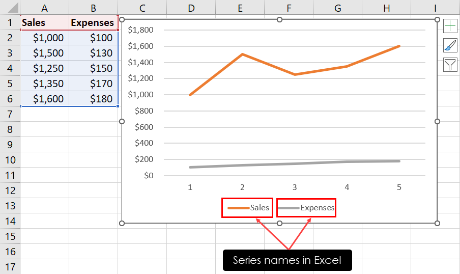
In Microsoft Excel, series names are labels given to different sets of data in a chart or graph. They help you identify and understand the information presented. These names are often based on the column or row data from your worksheet.

For example, if you have a chart displaying sales and expenses data for the month in your business, the series names could be Sales to represent revenue-earning instances and Expenses to represent payments made to vendors and service providers.

Series names make it easier for you to interpret the chart and recognize which data points belong to which category. You can customize these names to provide more clarity and context to your charts.

Also read: 7 Ways to Add Chart Axis Labels in Microsoft Excel

Reasons to Change Series Name in an Excel Chart

Here’s why you may want to rename the series names in Excel:

1. Renaming series allows you to enhance the clarity and comprehensibility of your Excel chart, aiding data interpretation.
2. Customized names ensure that the series titles are directly relevant to the data they represent, reducing ambiguity.
3. Meaningful series names provide valuable context, enabling you to better understand and communicate your data.
4. When you replace default series names with custom ones you increase the professionalism in your Excel reports.
5. Correcting default labels ensures that the series accurately represents your data, avoiding misinterpretation.
6. Your chart’s overall presentation and visual appeal are significantly improved with well-thought-out series names.
7. The aesthetics of your Excel chart benefit from well-crafted series names that contribute to a polished appearance.

Change Series Name From Edit Series Dialog

The Edit Series dialog box defines the name that should be displayed on the chart as well as the data embedded in it. So, you can use this tool to personalize the series name in your chart. Here are the steps you can try:

1. Click on the series names in the Legend Entry section of your chart.
2. Right-click on the series names and click on the Select Data option on the context menu.

3. The Select Data Source dialog will show up on your screen.
4. All the series names appear under the Legend Entries (Series) menu on the left-hand side.
5. Select any series in the list and click the Edit button.

6. You should now see the Edit Series dialog box.
7. Enter the new name inside the Series name field.
8. Click OK twice to save the changes made.

The above image shows the changed series names by following the mentioned steps.

Change Chart Series Name From Chart Design Tab

The Chart Design tab is the home to various chart customization commands like Chart Layouts, Change Colors, Data, Type, and Location. Inside the Data block of the Chart Design tab, you’ll find the Select Data tool.

Using Select Data, you can also quickly edit the series names without selecting the series names on the Excel chart. Find below the steps you can follow:

1. Highlight the chart to bring up the Chart Design tab.
2. Click the Chart Design tab.
3. Click the Select Data button inside the Data block.

4. You should now find the series names on the left-side menu on the Select Data Source dialog.
5. Select any series name and click the Edit button.

6. Now, you can enter the new series name inside the Series name field.
7. Click OK on the Edit Series and Select Data Source dialog boxes to implement the name series names.

The above is an example of a renamed series name.

Rename Series in Excel From Chart Filters

Another quick way to access the Edit Series dialog box is the Chart Filters tool.

Find below how to use it to change the series names in your Excel charts:

1. Click the Excel chart object on your worksheet.
2. Click the Chart Filters icon as shown in the above image.
3. A new context menu will appear with a tab for Values and below that the menu of Series.
4. Below the Series menu, hover the cursor over any series name that you want to edit.
5. Now, click the Edit Series icon on the right side of the series you’ve selected.

6. You should now see the Edit Series dialog.
7. From here, follow the steps mentioned earlier in this article to modify the series name.

Change Series Name Using Shortcut Keys

If you love working on your Excel worksheet with keyboard navigation to save time from mouse navigation, you must know how you can bring up the Select Data Source dialog so you can edit the series names.

Highlight the chart object and press Alt > JC > E to get to the Select Data Source dialog box.

From here, you can simply select the series name you want to edit.

Change Series Name in Excel From the Formula Bar

You can also use the Excel Formula Bar to edit the default series names on your chart to better alternatives. Here’s how:

1. Click on the series on the chart for which you want to change the name.
2. You should now see the chart formula that forms the series on your chart on the Excel Formula Bar.

3. The name of the series is at the beginning of the formula inside the parenthesis separated by two Excel separators or commas. For example, Sheet1!$B$1 in the current chart.
4. Delete this part and enter the custom series name, like Edit Name 2 in the place of Sheet1!$B$1.
5. Ensure you put the new series name within double quotes and don’t delete the two Excel separators.

6. Hit Enter to implement the series name change.

Change Series Names in Excel Using Excel VBA

If you want to automate the series name-changing process in Excel, you can write VBA scripts and execute those on the worksheet. Find below a VBA script that automatically changes the series names when run on a worksheet:

Sub ChangeSeriesName()
    Range("G18").Select
    ActiveSheet.ChartObjects("Chart 4").Activate
    Application.CutCopyMode = False
    ActiveChart.FullSeriesCollection(1).Name = "=""Sales"""
    ActiveChart.FullSeriesCollection(2).Name = "=""Expense"""
End Sub
 

To use the above script, follow these steps

1. Press the Alt + F11 keys together to launch the Excel VBA Editor.
2. There, click the Insert button.
3. Choose Module on the context menu.
4. Copy and paste the above script into the blank module.
5. Click Save and close the VBA Editor.

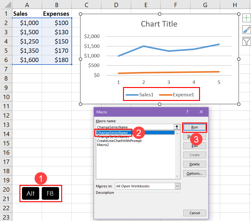
The above script will create the ChangeSeriesName VBA macro. Here’s how you can run it:

1. Press Alt + F8 to launch the Macro dialog box.
2. Select the ChangeSeriesName macro.
3. Click Run to execute the code.

Here’s how you can customize the script to work on your own worksheet:

• Replace Chart 4 in the code element ActiveSheet.ChartObjects("Chart 4").Activate with the chart name of your own worksheet. To locate the chart name, click the chart and look at the Name Box to the right of the Insert Function box.
• Put the new series name into the code element "=""Sales""" to change the name of the first series in the chart object. ActiveChart.FullSeriesCollection(1) represents the first series in the chart.
• Add more lines of the code element ActiveChart.FullSeriesCollection(3).Name = "=""Your Series Name""" if there are more series names that need changing. Just add numbers 3, 4, etc., according to the serial of the series names.

Note: Before applying this VBA macro in your Excel worksheet, create a backup copy of it. You won’t be able to undo changes when you use a VBA macro on your worksheet.

Also read: How To Use The VBA Code You Find Online

Conclusion

Changing series names in Excel is fairly easy when you follow any of the above-mentioned methods.

If you need to change one or two series names in a few charts, you can use methods like Edit Series, Chart Design Tab, Chart Filters, and the Formula Bar.

On the contrary, if there are many charts with many series names in each of those, try out the Excel VBA method.

If the above methods helped you in your data visualization journey on Excel, don’t forget to write a comment below. If you know another cool trick that I didn’t mention in this article, write about that in your comment.