You’re in the USA and your client is in the UK. By default, when you created your Excel worksheet and punched in a few dates, Excel formatted those in the US style.

Now, before sending the Excel report to your client, you must be wondering how to change the date format in Excel.

Adding days, dates, and years to your data adds a high-value context to the data. Your audience can see a timeline of a performance increase or decrease in the report you present.

Therefore, Excel allows you to include date, month, and year values. Also, it comes with a full-proof system of date formatting. Anyone from any part of the globe can use a date format they like and change that instantly without confusing the audience from a different part of the world.

Keep reading to learn all the easy and intuitive ways for changing the date format in Excel.

What Is an Excel Date Format?

An Excel date format is how data analysts and the audience see a date in Excel. For example, 7-4-2023 is July 4, 2023.

However, Excel keeps the dates in its database as continuing serial numbers starting from Jan 1, 1900, on Windows desktop systems and Jan 1, 1904, for Mac devices.

Excel understands the date July 4, 2023, as serial number 45111. This is known as the Microsoft Excel date-time code.

As a user, you don’t see dates this way. Excel formats the date in a Date, Month, and Year format set by your local machine.

For example, if your Windows 10 or 11 PC shows the Country or region as the United States in the Time & Language > Region section of the Settings app, Excel will format valid dates as DD-MM-YYYY, like 7-4-2023.

This is a highly efficient system since Excel can be used in any country or region and being a user you don’t need to stick to Microsoft’s date formatting. Rather, you can choose your own country’s date formatting rules or create custom formatting if needed.

Reasons to Change Date Format in Excel

• If you work in the off-shore office of a business or with foreign clients, you must change the date formats of your Excel worksheet according to the recipients’ preferences.
• Suppose, your business app accepts date formats in DD-MM-YYYY style but the Excel worksheet has date formatting in MM-DD-YYYY style. For compatibility reasons, you must change the date format before uploading the spreadsheet.
• You’re organizing and cleaning a raw dataset for your Excel worksheet. The dataset contains mentions of dates in different formats. By knowing how to change the formatting of dates in Excel, you can reformat all the dates to one format that your school, client, or business approves.
• If your Excel dataset is subject to further sorting, filtering, or other data analysis activities, you must standardize the date formatting system to one specific format throughout the spreadsheet.
• The date format 7/4/2023 may seem okay for the worksheet but when printing, if you use July 20, 2023, the readability increases a lot. To do this modification, you can apply an appropriate date formatting.
• Date format modification in Excel is also required to comply with legal and regulatory policies.

Change Date Format in Excel Using the Number Block

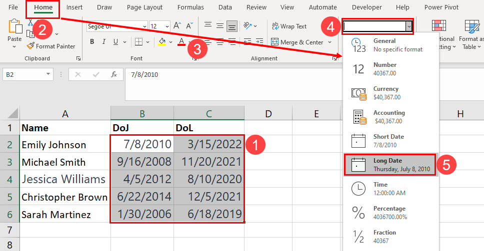
The obvious way to modify the existing date formatting to a different one in Excel is the Number commands block on the ribbon menu. Find below how it works:

1. Select a cell or column containing the date formats that need changing.
2. Go to the Home tab of Excel.
3. Navigate to the Number block.
4. Click the Number Format drop-down menu.
5. Choose a date formatting from the list, like Short Date or Long Date.

6. The date formatting changes will reflect in the selected dataset instantly.

Use Format Cells in Excel to Change Date Format

The Number Format drop-down menu only has two date formats. If you need more than just the Short and Long Date formats, you must use the Format Cells tool in Excel. Find below the quick steps to use this tool:

1. Highlight a date or a set of dates.
2. Press Ctrl + 1 on your keyboard to open the Format Cells dialog box.
3. Select the Date item under the Category column on the left.
4. Choose a date format under the Type column on the right.
5. Excel will display a preview of the chosen date format in the Sample field above the Type menu.
6. Click OK to save and apply the formatting to the selected dataset.

The above image shows the result of the date formatting applied using the Format Cells tool.

Change the Locale of a Date

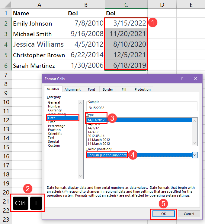
Suppose, your Excel worksheet contains dates in the US format, which is MM-DD-YYYY. Now, you need to quickly change the formatting to that of the UK formatting rule. Here’s how you can do it:

1. Select the date range on the worksheet.
2. Hit Ctrl + 1 to open the Format Cells dialog box.
3. Select a date format from the Type list.
4. Click the Locale drop-down menu below the Type list and select English (United Kingdom).
5. Click OK to apply the date formatting.

The above screenshot shows the result of the date formatting applied using the Format Cells > Locale drop-down menu.

Change Date Format Using a Custom Code

If you’re unable to get the date format you require in the Type list of the Format Cells dialog box, you can create the formatting style using a custom code. Here’s how it’s done:

1. Highlight the dates for which you need to modify the formatting.
2. Call the Format Cells dialog box by pressing the Ctrl + 1 keys.
3. Under the Category list, select Custom.
4. Now, type the date format you want as the following code:

mmmm-dd-yyyy

5. Check if the format is accurate by checking a display in the Sample field.
6. Click OK to apply the formatting.

7. Excel will instantly implement the formatting you created.

Find below a list of other custom formatting you can use:

Change Excel Date Formatting From a List of Texts

Sometimes, you may get a raw dataset containing date entries in text format. In this scenario, you can’t directly apply the above formatting techniques directly. First, you need to convert the text entries of dates into Microsoft Excel date-time codes.

Here are the steps you need to try:

1. Select a cell where you want to get the date-time code of a date.
2. Apply the following formula to the cell:

=DATEVALUE(B2)

3. Hit Enter to get the date code 40367.

4. If there are more date entries in text in the adjacent column, use the fill handle to apply the formula in other rows.

Once you’re done converting all the source dates into their corresponding date-time codes, follow these steps:

1. Select the date-time codes dataset.
2. Press Ctrl + 1 to bring the Format Cells dialog box.
3. Select the Date category.
4. Choose a Type from the right-side menu.
5. Click OK to apply the formatting.

Modify Date Format Using the TEXT Function

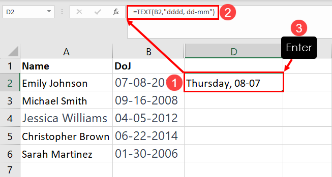
Suppose, there are dates in your Excel worksheet in the DD-MM-YYYY format. You just need to show a partial date, like the day and the date only, and not the year. You can do such custom formatting of dates using the TEXT function. Here’s how:

1. Choose a cell beside the source date data.
2. Enter the following formula into the cell:

=TEXT(B2,"dddd, dd-mm")

3. Hit Enter to get the date formatting Thursday, 08-07.

4. To apply the same formula to all the source dates, drag the fill handle in the column to the right.

Here’s how you can customize this function:

• B2 is the source data reference, so change it accordingly.
• Put the formatting you want using D, M, Y, AM, PM, HH, MM, etc., in double quotes.
• If you’re using multiple formation elements, like day name, month name, time, etc., separate the codes using a comma. For example, check this formula below:

=TEXT(B2,"mmmm, yyyy")

If you enter the above formula in any cell and provided that the B2 cell has a date entry, you’ll get an output as Month, YYYY (e.g., July, 2010).

Use Power Query to Change Date Format

Are you importing a large database with inconsistent date formatting that needs standard date formatting? You can use the Power Query tool in this scenario. Import the dataset into Power Query and follow these steps:

1. Click the Add Column tab and select the Custom Column button.
2. In the New column name field on the Custom Column wizard, type a column name.
3. Inside the Custom column formula field, enter the following formula:

=DateTime.ToText([DoJ],"dd-MM-yyyy")

4. Click OK to apply the formula.
5. You should see a new column in the Power Query tool with the date format you created.
6. Delete the unnecessary date columns.

7. Click File and choose Close & Load To.

8. On the Import Data dialog, choose Existing worksheet and select a cell.
9. Click OK to import the new date format column.

The above image shows converted date formats imported from Power Query.

Besides using formulas, you can also use the Transform tool in Power Query to choose a different date format for the added datasets, like Date Only.

Excel Changing Date Format Using a VBA Script

For advanced automation, you can use the following VBA script to change the date format for thousands of rows and columns in a flash. Make a backup copy of the worksheet before using the following macro. You won’t be able to undo any changes made by executing macros on Excel.

Sub ConvertDateFormats()
    Dim ws As Worksheet
    Dim cell As Range
    Dim targetRange As Range
    Dim convertedDate As Date
    Dim originalValue As String
    Dim desiredFormat As String
    
    Set ws = ThisWorkbook.Sheets("Sheet3")
    Set targetRange = ws.Range("B2:B6,C2:C6")
    desiredFormat = "dddd mm-yyyy" ' Change this format as needed
    
    For Each cell In targetRange
        originalValue = cell.Value
        If IsDate(originalValue) Then
            convertedDate = CDate(originalValue)
            cell.Value = Format(convertedDate, desiredFormat)
        End If
    Next cell
End Sub

To learn how to use this script in your own worksheet, read the following article:

How To Use The VBA Code You Find Online

Here’s how you can customize the above script according to your worksheet:

• Change Sheet3 to the actual worksheet name of your workbook.
• Change the cell ranges, like B2:B6 and C2:C6 according to your source datasets.
• To get a different date format change the existing format "dddd mm-yyyy" to the one you want, like "dd-mm-yyyy", "mmmm dd-yyyy", etc.

Change Date Format in Excel Using Office Scripts

If you need to automate the task on Excel for the web app, Excel VBA won’t work. You need to use Office Scripts. Find below the code and steps to use it:

1. Click the Automate tab and choose New Script.
2. Copy and paste the following Office Scripts code inside the Code Editor.

function main(workbook: ExcelScript.Workbook) {
	let selectedSheet = workbook.getActiveWorksheet();
	// Set range C2 on selectedSheet
	selectedSheet.getRange("C2").setFormulaLocal("=TEXT(B2,\"dddd mm-yyyy\")");
	// Auto fill range
	selectedSheet.getRange("C2").autoFill("C2:C6", ExcelScript.AutoFillType.fillDefault);
}

3. Click the Save script button and select the Run button.
4. Excel will convert the source date formats to a custom output as per the code.

Here’s how to modify the code:

• Change C2 to another destination cell as per your worksheet.
• In the TEXT formula, B2 is the source date value. Change this cell address as per your own dataset.
• Also in this formula, enter the date format you want by replacing this code "dddd mm-yyyy\".
• If you’re using AutoFill, change the cell ranges C2:C6 according to your worksheet.

Conclusions

So these are some of the common ways to change the date format in Excel. If your dataset is small, you can use manual methods like the Number block in the Excel Ribbon menu or the Format Cells dialog box.

Contrarily, if your dataset is medium to large and you want automation in the task, use the methods which involve Excel VBA or Office Scripts.

Suppose you’re importing datasets from an external server or third-party database application, use the Power Query tool to modify the date formats in Excel.