Looking for ways to pull data from another worksheet or workbook in Excel to build tables, charts, etc.? Keep reading to learn some quick and efficient ways.

Besides being the leading data analytics and visualization software, Excel is also a robust database management tool. It offers various ways to aggregate data from different worksheets, workbooks, and workbooks stored on a server or cloud storage.

Therefore, you can make dynamic dashboards and tables to get data insights from raw data. You don’t need to keep the raw data on the same worksheet where you keep your data visualizations. Workbook and worksheet referencing make this possible.

Find below multiple ways to pull data from another sheet or workbook using manual and automated methods.

Why Pull Data From Another Sheet in Excel

Pulling data from a different worksheet or workbook is particularly helpful when it becomes impractical to maintain extensive worksheet models within a single workbook. The technique helps you to:

1. You can establish links between workbooks used by various users or departments and incorporate relevant data into a summary workbook.
2. Enter all data into one or more source workbooks and then create a separate report workbook that utilizes external references to extract only the required data.
3. By breaking down a complex model into interconnected workbooks, you can work on specific aspects without opening all related sheets.

Using Sheet and Cell References

You can pull data from different worksheets and workbooks easily if you follow the following convention of Excel to reference the source:

1. When referencing a worksheet in the same workbook, input the name of the worksheet followed by an exclamation mark. For example, if you’re importing a table from the cell range A1:B4 in Sheet2 to Sheet1, type the following syntax in the destination cell on Sheet1.

=Sheet2!A1:B4

2. If there is any space in the name of the worksheet, type the name as is and then put it into single quotes. For example, the worksheet name Sheet 2 must be referred to as ='Sheet 2'! A1:B4.
3. When referencing a workbook, put the workbook name within square brackets and then reference the target worksheet in that workbook as is. For example, if you’re pulling data from another workbook pulldata2.xlsx to pulldata.xlsx, then highlight a destination cell and enter this syntax:

=[pulldata2.xlsx]Sheet1!A1:B4

If you’re using a dated Excel desktop app like Excel 2007, Excel 2010, etc., you must hit Ctrl + Shift + Enter to reference a worksheet or workbook. Because these reference formulas work as Excel array formulas.

However, if you’re using Excel for the Web or Excel for Microsoft 365 desktop app, you can simply hit the Enter key.

Pull Data From the Same Workbook

Find below the instructions to pull data from a worksheet in the same workbook using the INDEX and MATCH formulas. This example explains how to use a formula with worksheet referencing.

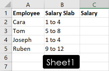
1. In Sheet1, I got employee names, salary slabs, and salary columns. I must import the salaries of the employees from a database of salary slabs and actual salaries in Sheet2.

2. In cell C2, I’m entering the following formula that uses INDEX and MATCH to pull the correct data from Sheet2 to Sheet1:

=INDEX(Sheet2!$A$2:$A$4,MATCH(B2,Sheet2!$B$2:$B$4,0))

3. Now, I can drag the fill handle down column C to populate salaries for other employees.

When using the formula in your own dataset, modify it as outlined below:

• Sheet2!: Change it to the exact worksheet name in your workbook.
• $A$2:$A$4: Modify the cell range according to the dataset that needs indexing.
• B2: It’s the reference data by matching which Excel will pull data from the indexed dataset.
• $B$2:$B$4: This is the look-up value or array. Modify it according to your own dataset.

Pull Data From a Different Workbook

When you’re pulling data from a different workbook than the one you’re working on, you just need to include its name in the same formula shown above. Now, there could be two situations. One, where you’ve opened the source workbook, and the other where you didn’t open the source workbook.

If the source workbook is also open, use this formula:

=INDEX([pulldata2.xlsx]Sheet1!$A$2:$A$4,MATCH(B2,[pulldata2.xlsx]Sheet1!$B$2:$B$4,0))

If the source Excel file isn’t open but it’s on the same computer, use the following formula instead:

=INDEX('C:\[pulldata2.xlsx]Sheet1'!$A$2:$A$4,MATCH(B2,'C:\[pulldata2.xlsx]Sheet1'!$B$2:$B$4,0))

The difference in the above two formulas is the mention of the complete location of the source workbook in the internal storage of the PC.

When creating the link between two workbooks for the first time, keep both of them open and use the first formula that doesn’t show the address of the source Excel workbook. Now, the next time, if you keep the source workbook closed, Excel will add the directory address to the formula if the workbook isn’t open.

Pull Data Using Fill Handle

Another easy way to pull data without any formula in Excel is by using the fill handle. Suppose, you need to often copy a dataset from one worksheet to the other.

Here’s how you can do it in a few clicks without remembering any worksheet or workbook referencing convention in Excel:

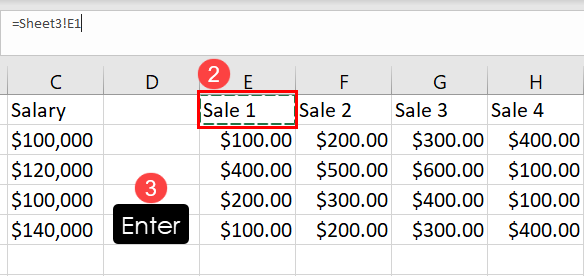
1. Double-click the destination cell and enter an equal sign (=).
2. Now, go to the source worksheet or workbook and highlight the starting cell of the table or dataset.
3. Hit Enter.
4. Excel will take you to the destination worksheet and pull the selected cell data from the source.

5. Now, use the fill handle vertically to populate the data from the source worksheet or workbook.

6. Then, drag the fill handle horizontally to get the rest of the dataset or table.

7. You might see some cells containing the number 0. This represents the blank cells in the source worksheet or workbook.
8. Use the fill handle again to adjust the cell ranges horizontally and vertically to erase zeroes.

Sub RemoveZeros()
    Dim rng As Range
    Dim cell As Range

    Set rng = ActiveSheet.UsedRange 
    For Each cell In rng
        If IsNumeric(cell.Value) And cell.Value <> "" Then
            If cell.Value = 0 Then
                cell.Value = ""
            End If
        End If
    Next cell
End Sub

Alternatively, use the above Excel VBA code to get rid of zeroes.

Here’s how you can quickly use the above code:

1. Right-click on the worksheet name.
2. Click View Code on the context menu.

3. Copy and paste the above VBA script inside the blank module.
4. Click the Save button.

5. Now, press Alt + F8 to bring up the Macro dialog box and run the RemoveZeros macro.

Pull Data Using Named Range

Named range in Excel allows you to define a name for a table or dataset within a workbook. Now, you can refer to the name instead of the cell range to pull data from a different worksheet or workbook. Find below the steps to creating and linking a named range to import data to a worksheet:

1. Highlight the dataset in the source worksheet or workbook.
2. Click the Formulas tab on the Excel ribbon menu.
3. Inside the Defined Names commands block, click Define Name.
4. In the New Name dialog box, enter a name you can remember for the highlighted dataset into the Name field.
5. Click OK to complete the process.

=puuldata.xlsx!sales

6. Now, go to the destination cell in a worksheet and enter the above formula.

7. Press Enter or Ctrl + Shift + Enter to pull data from another sheet in Excel.

Copy Data From Another Sheet

The easiest way to pull data from another worksheet or workbook is the copy-paste method. However, this method might not be convenient when you need to pull a large dataset. Not to mention, manual copying and pasting comes with the risk of human error.

Find below two ways to automate the copy-paste process in Excel to pull data from a source worksheet:

Copy Data Between Worksheets Using VBA

1. Press Alt + F11 to call the Excel VBA Editor interface.
2. Click the Insert menu and choose Module.

Sub PullDataFromSheet4ToSheet3()
    Dim sourceSheet As Worksheet
    Dim destinationSheet As Worksheet
    Dim sourceRange As Range
    Dim destinationCell As Range
    Set sourceSheet = ThisWorkbook.Worksheets("Sheet4")
    Set destinationSheet = ThisWorkbook.Worksheets("Sheet3")
    Set sourceRange = sourceSheet.Range("A1:H5")
    Set destinationCell = destinationSheet.Range("A1")
    sourceRange.Copy destinationCell
End Sub

3. Into the new module, copy and paste this VBA script:
4. Click the Save button and close the VBA Editor.

5. Now, bring up the Macro dialog box by pressing Alt + F8 keys.
6. Select the PullDataFromSheet4ToSheet3 macro and hit the Run button.

Excel will copy the source data into the destination worksheet instantly. Find below how to customize the VBA macro to make it work for your worksheet:

• Sheet4: It’s the source of data so modify the sheet name.
• Sheet3: It’s the destination where Excel will pull data from the source.
• A1:H5: This is the cell range of the source data that Excel will copy. Change it to include more or less data according to your source worksheet.
• A1: It’s the first cell in the destination worksheet from which Excel will start pasting the copied data. You can modify it if you want to.

Copy Data Between Sheets Using Office Scripts

Suppose you want to automate the pull data process from one worksheet to another on Excel online app. Since VBA won’t work there, you can use Office Scripts. Find below the steps you should try:

1. Go to the destination worksheet and click Automate on the Excel ribbon.
2. Click New Script inside the Scripting Tools commands block.
3. The Code Editor panel will appear on the right side of Excel.

function main(workbook: ExcelScript.Workbook) {
	let sheet3 = workbook.getWorksheet("Sheet3");
	let sheet4 = workbook.getWorksheet("Sheet4");
	let selectedSheet = sheet3; // Set Sheet3 as the selected sheet

	// Paste to range E1 on Sheet4 from range E1:H5 on the selectedSheet (Sheet3)
	sheet4.getRange("E1").copyFrom(selectedSheet.getRange("E1:H5"), ExcelScript.RangeCopyType.all, false, false);
}

4. There, copy and paste the above Office Scripts code.
5. Click the Save script button to save the code.
6. Now, hit the Run button to pull data from another worksheet in Excel automatically.

Here’s how you can personalize the above Office Scripts code.

• Change all the occurrences of Sheet3 with the actual worksheet name of the source data.
• Similarly, modify all the occurrences of Sheet4 according to the destination worksheet name.
• Replace "E1" in the code element sheet4.getRange("E1") with a cell address from which you want to start pasting the source data.
• Replace the cell range "E1:H5" in the code element selectedSheet.getRange("E1:H5") with the actual source data range, like "A1:F100", "B2:E10", etc.

Office Scripts is only available on Microsoft 365 subscription Business Standard or better. Also, you need an internet connection if you want to use Office Scripots in Excel for Microsoft 365 desktop app. If you see the Automate tab on Excel, you can use Office Scripts.

Pull Data From Another Sheet Using Power Query

Power Query is another cool database querying tool of Excel that lets you import data from different worksheets of the same workbook or from a different workbook.

When pulling data from Excel files using Power Query, you can make the process more efficient by using named ranges. Refer to the named range creation process explained above to give a name to the source dataset or table.

Once you’ve got the Defined Name you need, follow these steps:

1. Go to the destination worksheet and click the Data tab.
2. Hit the Get Data button and choose From Excel Workbook.

3. Navigate to the source workbook and select it in the Import Data dialog box.
4. Click Import to load the content of the workbook in the Navigator dialog box.

5. Select the named range from the left-side panel.
6. Now, click the drop-down arrow of the Load button and choose Load To.

5. Select Existing worksheet on the Import Data dialog box and click OK.

Excel will instantly import the selected named range as a table with active filters. Select all the column headers and press Ctrl + Shift + L to deactivate filters.

Conclusions

So, now you know all the cool and intuitive methods to pull data from another sheet in Excel. You can also apply these steps to import data from a worksheet in a different workbook on your computer.

If you’re just starting your Excel journey, you can use the sheet and cell referencing method or the fill handle method. These are suitable for small datasets.

If you’re an expert-level Excel user and don’t mind writing a few lines of codes, use the Excel VBA and Office Scripts-based methods. These allow you to automate the whole process.

Finally, if you need to transform the source data into an organized structure before importing into the active worksheet, use the Power Query-based method. It comes with a visual interface so you can perform complex data management activities without writing codes.