Transposing data is a very common task regardless what program you’re working in with your data.
Sooner or later you’ll come across the need in Excel too!
In this post, I’ll show you 3 easy ways to do this in Excel.
Video Tutorial
What Does Transposing Data Mean?

To transpose literally means to cause two or more things to change places with each other.
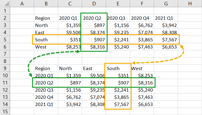
When dealing with data, this means you want to change rows into columns and change columns into rows like in the above example.
Essentially, this means flipping the data on the diagonal axis that goes from the top left corner to the bottom right corner.
Why You Might Want to Transpose Your Data
The example used in this post contains a small set of sales data by period and region. The period is going across the columns and the region is going down the rows.
You might want to change this because as time goes on, this data set will get quite wide.
The region is better off going across the columns as there won’t be an increasing number of regions, this will be fixed at the 4 regions and the data will be easier to see in one page as the data grows.
Transpose Data with Paste Special Command
The first method is to use the transpose option in the paste special command menu.
This method is quick and easy, but it’s best suited when you want to transpose your data as a one off action and don’t need this transformation as part of a repeated process that needs to be done monthly, weekly or even daily.

Copy the data you want to transpose.
- Select the data you want to transpose.
- Go to the Home tab.
- Click on the Copy command.
You can also select the data then use the Ctrl + C keyboard shortcut to copy the data instead of using the ribbon commands.

Paste the data using the transpose command.
- Select the cell where you want the transposed data. This will be the upper left of where the data will go.
- Press the lower part of the Paste button in the Home tab for more paste options.
- Select the Paste Transpose command.
This will result in the transposed data being pasted in the sheet.

You can also perform this transpose command from the Paste Special menu. After you copy the data you can use the Ctrl + Alt + V keyboard shortcut to open the Paste Special menu.
Check the Transpose option then press the OK button to paste the transposed data.
Transpose Data with the TRANSPOSE Function
There is actually a function in Excel to transpose data, but before the introduction of dynamic arrays in Microsoft 365 it was not really that interesting of a function.
You couldn’t use it to return transposed data and could only really use it to transpose data for use within a calculation to return a scalar value like from a matrix multiplication.
Syntax
= TRANSPOSE ( Range )- Range – This is the range of data you want to transpose.
The TRANSPOSE function is very simple. It takes one argument which is the range of data you want to transpose.
TRANSPOSE Function as a Dynamic Array
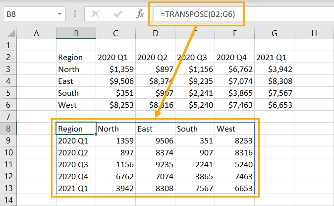
If you’re using the TRANSPOSE function in Microsoft 365, then it’s very easy to use and the results will automatically spill as an array of values.
This is a great option if you want the transposed results to update when you change the source data.

= TRANSPOSE ( B2:G6 )All you need to do is type the above formula into the cell where you want the transposed data. The data will spill down and to the right of the cell with the formula.
Unlike the copy and paste method to transpose, this is dynamic. If you change anything in the source range, it will automatically update in the transposed results.
It is also very easy to update the source range in the formula if the source data grows in size.
TRANSPOSE Function with Ctrl Shift Enter
If you don’t have dynamic arrays, then using the TRANSPOSE function to get a range of transposed data can still be done, but it’s more difficult and is less flexible to change.

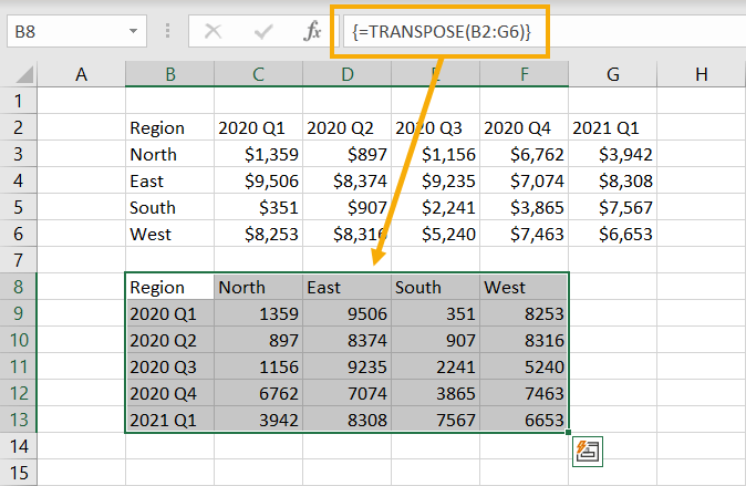
You will first need to select the correct output range for the transposed data. This example data has 5 rows and 6 columns, so you will need to select a range of 6 rows and 5 columns before typing out the formula.
In general, if your data is N rows and M columns, then you have to select a range of M rows and N columns before entering the formula.

Instead of pressing Enter like usual to enter the formula, press Ctrl + Shift + Enter.
This results in an array formula that spans the entire selected range. Notice the formula now has a set of curly braces around it to indicate it is an array formula.
These are not flexible and if the source data grows then you will need to delete the array formula and re-enter it with a new increased range.
Transpose Data with Power Query
This is the method of choice if you need to repeatedly get data from some source and transpose it.
The first step is to make sure your data is inside an Excel table. This way you can import the data into power query and perform the transformation.

Select the table with the data you want to transpose and then go to the Data tab and press the From Table/Range command.
This will open up the power query editor.

Some of the data you might want to transpose will be in the column headings. To include this you will first need to demote the column headings to a row in the data.
- Go to the Transform tab.
- Click on the lower part of the Use First Row as Headers command to reveal more options.
- Select the Use Headers as First Row command.

In the power query editor go to the Transform tab and select the Transpose command.

After the data has been transposed, you will probably also want to promote the first row (which previously was the first column) to the column headers.
Go to the Transform tab and press the Use First Row as Headers command.
Now the data is fully transposed and you can go to the Home tab and Close and Load the data into an Excel worksheet of your choice.
The great thing about this option is you can easily add/remove rows and columns to/from the source table. When you press the Refresh button in the Data tab these changes will be reflected in the transposed output from power query.
Conclusions
There you go, 3 easy ways to transpose your data in Microsoft Excel!
Since the introduction of dynamic arrays, my favourite method is using the TRANSPOSE function. It’s quick, easy and will automatically update when you change your source data.
Do you have any favourite, or know a method that wasn’t listed? Let me know in the comments!
 👉 Find out more about our Advanced Formulas course!

![6 Ways to Count Colored Cells in Microsoft Excel [Illustrated Guide]](http://cdn-5a6cb102f911c811e474f1cd.closte.com/wp-content/uploads/2021/08/Count-Coloured-Cells-in-Excel.png)


0 Comments