When using data in Excel that has been imported from another source, the text is often not how you wish to see it.

You may find that product references consist of a product code, code reference, and product size all concatenated into one piece of text which appears in one cell within the worksheet.

Your requirement is that you want to split the relevant sections of the text string so that they all appear in individual cells in your worksheet.

This may be because you want to sort or group by a particular section of text. You may also want to use other formulae on that particular split section. For example, you may want to do a lookup on another table of data, using that section of text as the lookup value. This would be impossible with the data in its original form.

If you are using the data in a pivot table, you may require a separate field that has the split data in order to allow filtering or consolidation.

This article describes seven ways in which you can extract the first or last N characters from a string of text data in Microsoft Excel.

Sample Data Used in this Post

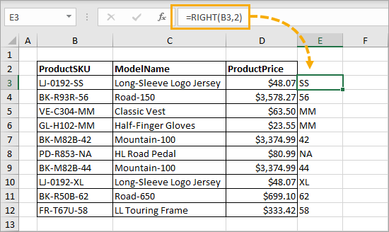
The examples in this post will extract the first and last 2 characters from the ProductSKU in the above set of small product data. The first 2 characters in the SKU contains the product category code and the last 2 characters contains the product size.

Extract Characters with LEFT and RIGHT functions

Excel has several useful functions for splitting strings of text to get at the actual text that you need.

LEFT Function

Syntax:

LEFT ( Text, [Number] )

• Text – This is the text string that you wish to extract from. It can also be a valid cell reference within a workbook.
• Number [Optional] – This is the number of characters that you wish to extract from the text string. The value must be greater than or equal to zero. If the value is greater than the length of the text string, then all characters will be returned. If the value is omitted, then the value is assumed to be one.

This will return the specified number of characters from the text string, starting at the left-hand side of the text. It will extract the first specified number of characters from the text.

RIGHT Function

Syntax:

RIGHT ( Text, [Number] )

The parameters work in the same way as for the LEFT function described above.

This will return the specified number of characters from the text string, starting at the right-hand side of the text. It will extract the last specified number of characters from the text.

Extract Characters with Text to Column

Text to Columns allows you to split a column into sections by defining fixed limits to your text section. To use this methodology:

1. Select all the data in the ProductSKU column in the sample data.
2. Click on the Data tab in the Excel ribbon.
3. Click on the Text to Columns icon in the Data Tools group of the Excel ribbon and a wizard will appear to help you set up how the text will be split.
4. Click on the Fixed Width option button.
5. Click on Next for the next step of the wizard.

In the second step, in the Preview Window, click on the measuring bar in Data Preview where you want to divide the text. This will display a vertical line showing the separation. Do this again for the right-hand characters.

Click on Next to go to the final step of the wizard.

Set the destination cell to E3, so that existing data does not get overwritten.

Click Finish and your data will be imported into three columns commencing at cell E3.

Your worksheet will now look like above with the results split into separate cells.

Extract Characters with Flash Fill

This Flash Fill methodology allows you to enter a couple of examples into the cells where you want your split data to appear. Excel then works out what data is needed in the column based on your examples.

The disadvantage of this methodology is that the examples dictate how many characters will be extracted. This works well if it is always a uniform number, but in some cases, it may not be, in which case this will not work.

To use Flash Fill, you need to enter at least three examples of the text that you wish to see.

You can also activate Flash Fill in the Data Tools group of the Data tab on the Excel ribbon or by using the Ctrl + E keyboard shortcut.

Excel will then automatically fill in the remaining data based on your examples.

Extract Characters with VBA

VBA is the programming language that sits behind Excel and allows you to write your own code to manipulate data, or to even create your own functions.

To access the Visual Basic Editor (VBE), you use ALT + F11.

Sub SplitText()
Dim N As Integer
For N = 3 To 12
    ActiveSheet.Cells(N, 5).Value = Left(Cells(N, 2), 2)
Next N
End Sub

Inside the visual basic editor.

1. Click on Insert in the menu bar.
2. Click on Module and a new pane will appear for the module.
3. Paste in the above code.

Your window will now look like above.

Put the cursor anywhere within the code procedure and then press F5 to run the code.

The code loops through the values of 3 to 12, which are the row numbers for the sample data. It enters the first two characters of the text found at the row number N and column 2 into column 5 (column E).

This is very simple VBA code, and it has the disadvantage that it only takes the first two characters of the product code. If the product code is longer then the wrong result will be produced.
However, the code could be extended to search for the delimiter character (-) and then take the number of characters up to that point.

Extract Characters with Power Query

Power Query is a useful tool in Excel for manipulating data, and it can easily be used to split a column of data into sections.

First, you need to convert your data into an Excel table.

Create a From Table/Range query.

1. Select a cell inside the table.
2. Go to the Data tab
3. Click on From Table/Range in the Get & Transform Data group.

This will open up the power query editor which will allow you to transform the data.

1. Click on the ProductSKU column.
2. Click on the Add Column tab of the power query editor.
3. Click on Extract in the From Text group.
4. Select First Characters in the drop-down.

A pop-up window will be displayed. Enter 2 into the Count box. Click on OK and a new column called First Characters will be added. Double-click on the new column header and rename it to Category.

= Table.AddColumn(#"Changed Type", "First Characters", each Text.Start([ProductSKU], 2), type text)

This will result in the above M code formula.

If you need the last 2 characters, then click on Last Characters in the Extract drop-down.

= Table.AddColumn(#"Inserted First Characters", "Last Characters", each Text.End([ProductSKU], 2), type text)

It will result in the above M code formula.

Click on Close and Load in the Close group on the Home tab of the ribbon, and a new worksheet will be added to your workbook with a table of the data in the new format.

Extract Characters with a Power Pivot Calculated Column

You can also use a Power Pivot Table to show the first two characters of the Product Code.

To do this you need to convert your data into an Excel table.

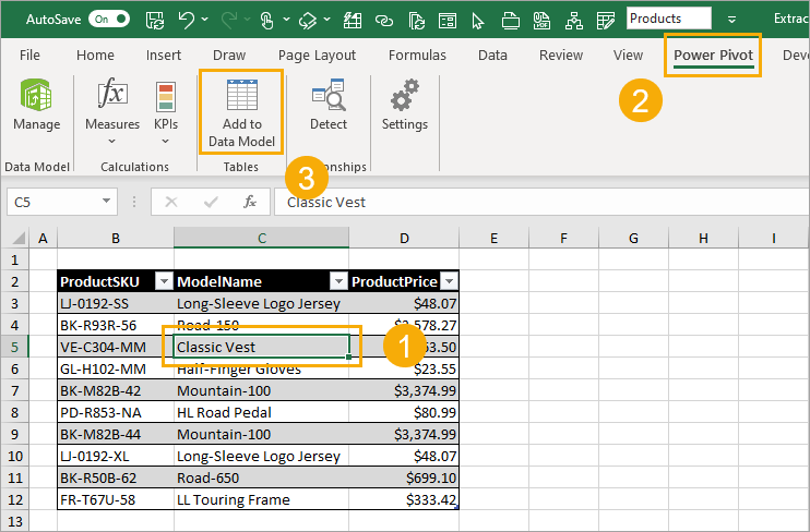
To import your data into Power Pivot:

1. Select a cell inside the table.
2. Go to the Power Pivot tab. If you don’t see the Power Pivot tab, you can install it by going to the Data tab and clicking on Manage Data Model.
3. Select Add to Data Model.

This will open the Power Pivot add-in with the table loaded. You can open this any time from the Power Pivot tab by selecting Manage in the Data Model group in the Excel ribbon.

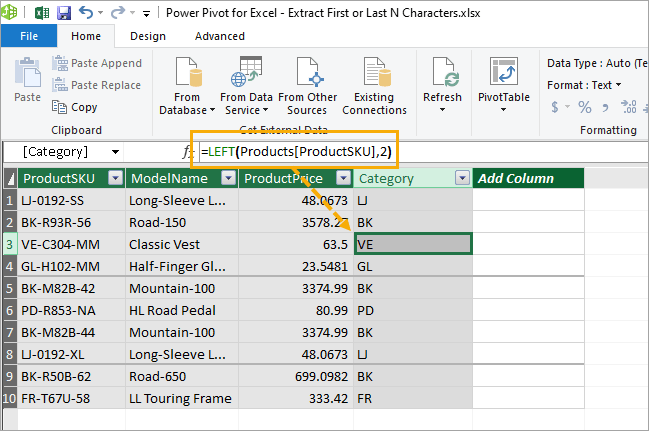
Right-click on the header for the Add Column and click on Rename Column in the pop-up menu. You can also double click on the column to rename it. Then you can rename this to something like Category.

= LEFT(Products[ProductSKU], 2)

Select any cell inside the new Category column and insert the above formula into the formula bar. Regardless of which cell you enter this formula in, it will propagate throughout the entire column.

The Category column now shows the first two characters of the product code.

= RIGHT(Products[ProductSKU], 2)

You can do the same with the above formula for the last 2 characters.

Click on the Pivot Table icon in the ribbon and click on Pivot Table in the pop-up menu in order to turn your source data into a spreadsheet pivot table.

Specify the location of your pivot table in the first pop-up window and click OK. If the Pivot Table Fields pane does not automatically display, right click on the pivot table skeleton and select Show Field List.

Now you can summarise your data by Category or Size.

In the Pivot Table Fields Pane, double click on your data source name e.g. Products and this will show the available fields. Check all the boxes to use all fields in your pivot table.

In the Rows box, drag the Category field to the top of the list so that the pivot table will summarise by different categories.

All the normal pivot table functionality is available in terms of re-naming columns, formatting numbers, etc.

Extract Characters with a Power Pivot Measure

To use a measure to split the field ProductSKU, you use the same data source instructions as for the Calculated Column methodology shown above.

When you click on the Power Pivot tab and click on the Manage icon, you can enter a Measure into the Power Pivot Manager window.

This window is divided into two sections. The top section shows the source data in the table, and the bottom section shows the measures. These are formulae that use the data in the table, and create a calculated field that can be used within the pivot table.

Category List :=
CONCATENATEX (
    VALUES ( Products[Category] ),
    Products[Category],
    ", "
)

Select the first cell in the measures section and enter the above formula in the formula bar.

A measure always needs to return a scalar value. This is why the CONCATENATEX function is used first in order to aggregate the results of the calculated columns created from the LEFT or RIGHT functions. If the CONCATENATEX function is not present, then this will return an error value and cannot be used in the pivot table.

Click on the Pivot Table icon in the ribbon, and follow the instructions to create the pivot table as shown above in the calculated column example.

In the Pivot Table Fields list, there is now a calculated field called Category, shown with fx in front of it. This returns the first two characters of the field ProductSKU.

Because a measure is always a calculated field, it can only be included as a value, even though it actually returns a text value in this case. It cannot be used as a filter or as a row or column name.

This is a huge disadvantage overusing a calculated column in the Power Pivot.

Conclusion

There are many ways to get the first or last few characters from your text in Excel.

You can use formula, text to column, flash fill, VBA, Power Query, or Power Pivot.

Which one do you prefer?