Not all data is numeric, so when creating random sets of sample data it can be very useful to know how to randomly select some text data from a list.
In that post, I showed you a way to randomly select from a list using the RANDBETWEEN function. This method produced an equal chance of selecting each item in the list. But what if we want to weight those probabilities of selection so that some items are more frequently selected than others?
With this method we can create the probability distribution of an item being selected.
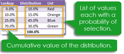
In this example, we are going to select from a list with 4 items. This is what’s in our Distribution and List columns in the above table.
- Red – We want this to be selected 10% of the time.
- Orange – We want this to be selected 15% of the time.
- Blue – We want this to be selected 45% of the time.
- Green – We want this to be selected 30% of the time.
Note that our probabilities of selection need to add to 100%! Our Lookup column is then just the running total of the Distribution Column. This will be the key to our random selection.
Generic Formula for Random Selection
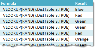
We will use a VLOOKUP with an approximate match to lookup an item from our list.
- DistTable – This is our table shown above which contains our distribution and list of items to select from.
- 3 – We want to return the result from the third column of the DistTable which contains the list items.
- TRUE – This tells Excel to use an approximate match for the VLOOKUP.
How Does This Work?
RAND() is an Excel function with no input parameters that will return a uniformly distributed random number between 0 and 1. We use this random number between 0 and 1 as the value to lookup in our DistTable. Since this lookup value is random, the result returned from the List column will also be random.
For example, if RAND() returned 0.1156 then the approximate match would be the 10% in the Lookup column because 10% <= 0.1156 < 25%. VLOOKUP would then return Orange since this is the 3rd column in the 10% row.
Let’s Check if it Works!
Let’s check if it works! If we use this formula 100 times, we should see approximately 10 Red, 15 Orange, 45 Blue and 30 Green results.

We can easily create a pivot table to count the number of items of each from the list, and we can even create a nice looking PivotChart to show the results. Our results look pretty close to the distribution we created. According to the law of large numbers, the larger the number of selections we make then the closer we will get to our intended distribution.


 👉 Find out more about our Advanced Formulas course!


0 Comments